Chapter 6 Interpreting Regression Results
Chapter Preview. A regression analyst collects data, selects a model and then reports on the findings of the study, in that order. This chapter considers these three topics in reverse order, emphasizing how each stage of the study is influenced by preceding steps. An application, determining a firm’s characteristics that influence its effectiveness in managing risk, illustrates the regression modeling process from start to finish.
Studying a problem using a regression modeling process involves a substantial commitment of time and energy. One must first embrace the concept of statistical thinking, a willingness to use data actively as part of a decision making process. Second, one must appreciate the usefulness of a model that is used to approximate a real situation. Having made this substantial commitment, there is a natural tendency to “oversell” the results of statistical methods such as regression analysis. By overselling any set of ideas, consumers eventually become disappointed when the results do not live up to their expectations. This chapter begins in Section 6.1 by summarizing what we can reasonably expect to learn from regression modeling.
Models are designed to be much simpler than relationships among entities that exist in the real world. A model is merely an approximation of reality. As stated by George Box (1979), “All models are wrong, but some are useful.” Developing the model, the subject of Chapter 5, is part of the art of statistics. Although the principles of variable selection are widely accepted, the application of these principles can vary considerably among analysts. The resulting product has certain aesthetic values and is by no means predetermined. Statistics can be thought of as the art of reasoning with data. Section 6.2 will underscore the importance of variable selection.
Model formulation and data collection form the first stage of the modeling process. Students of statistics are usually surprised at the difficulty of relating ideas about relationships to available data. These difficulties include a lack of readily available data and the need to use certain data as proxies for ideal information that is not available numerically. Section 6.3 will describe several types of difficulties that can arise when collecting data. Section 6.4 will describe some models to alleviate these difficulties.
6.1 What the Modeling Process Tells Us
Model inference is the final stage of the modeling process. By studying the behavior of models, we hope to learn something about the real world. Models serve to impose an order on reality and provide a basis for understanding reality through the nature of the imposed order. Further, statistical models are based on reasoning with the available data from a sample. Thus, models serve as an important guide for predicting the behavior of observations outside the available sample.
6.1.1 Interpreting Individual Effects
When interpreting results from multiple regression, the main goal is often to convey the importance of individual variables, or effects, on an outcome of interest. The interpretation depends on whether or not the effects are substantively significant, statistically significant and causal.
Substantive Significance. Readers of a regression study first want to understand the direction and magnitude of individual effects. Do females have more or less claims than males in a study of insurance claims? If less, by how much? You can give answers to these questions through a table of regression coefficients. Moreover, to give a sense of the reliability of the estimates, you may also wish to include the standard error or a confidence interval, as introduced in Section 3.4.2.
Recall that regression coefficients are estimates of partial derivatives of the regression function
\[ \mathrm{E~}y = \beta_0 + \beta_1 x_1 + \ldots + \beta_k x_k. \]
When interpreting coefficients for continuous explanatory variables, it is helpful to do so in terms of meaningful changes of each \(x\). For example, if population is an explanatory variable, we may talk about the expected change in \(y\) per 1,000 or one million change in population. Moreover, when interpreting regression coefficients, comment on their “substantive” significance. For example, suppose that we find a difference in claims between males and females but the estimated difference is only 1% of expected claims. This difference may well be statistically significant but not economically meaningful. Substantive significance refers to importance in the field of inquiry; in actuarial science, this is typically financial or economic significance but could also be non-monetary, such as effects on future life expectancy.
Statistical Significance. Are the effects due to chance? The hypothesis testing machinery introduced in Section 3.4.1 provides a formal mechanism for answering this question. Tests of hypotheses are useful in that they provide a formal, agreed-upon standard, for deciding whether or not a variable provides an important contribution to an expected response. When interpreting results, typically researchers cite a \(t\)-ratio or a \(p\)-value to demonstrate statistical significance.
In some situations, it is of interest to comment on variables that are not statistically significant. Effects that are not statistically significant have standard errors that are large relative to the regression coefficients. In Section 5.5.2, we expressed this standard error as
\[\begin{equation} se(b_{j}) = s \frac{\sqrt{VIF_{j}}}{s_{x_{j}} \sqrt{n-1}}. \tag{6.1} \end{equation}\]
One possible explanation for a lack of statistical significance is a large variation in the disturbance term. By expressing the standard error in this form, we see that the larger the natural variation, as measured by \(s\), the more difficult it is to reject the null hypothesis of no effect (\(H_0\)), other things being equal.
A second possible explanation for the lack of statistical significance is the high collinearity, as measured by \(VIF_j\). A variable may be confounded with other variables such that, from the data being analyzed, it is impossible to distinguish the effects of one variable from another.
A third possible explanation is the sample size. Suppose that a mechanism similar to draws from a stable population is used to observe the explanatory variables. Then, the standard deviation of \(x_j\), \(s_{x_j}\), should be stable as the number of draws increases. Similarly, so should \(R_j^2\) and \(s^2\). Then, the standard error \(se(b_j)\) should decrease as the sample size, \(n\), increases. Conversely, a smaller sample size means a larger standard error, other things being equal. This means that we may not be able to detect the importance of variables in small or moderate size samples.
Thus, in an ideal world, if you do not detect statistical significance where it was hypothesized (and fully expected), you could: (i) get a more precise measure of \(y\), thus reducing its natural variability, (ii) re-design the sample collection scheme so that the relevant explanatory variables are less redundant and (iii) collect more data. Typically, these options are not available with observational data but it can nonetheless be helpful to point out the next steps in a research program.
Analysts occasionally observe statistically significant relationships that were not anticipated—these could be due to a large sample size. Above we noted that a small sample may not provide enough information to detect meaningful relationships. The flip side of this argument is that, for large samples, we have an opportunity for detecting the importance of variables that might go unnoticed in small or even moderate size samples. Unfortunately, it also means that variables with small parameter coefficients, that contribute little to understanding the variation in the response, can be judged to be significant using our decision-making procedures. This serves to highlight the difference between substantive and statistical significance—particularly for large samples, investigators encounter variables that are statistically significant but practically unimportant. In these cases, it can be prudent for the investigator to omit variables from the model specification when their presence is not in accord with accepted theory, even if they are judged statistically significant.
Causal Effects. If we change \(x\), would \(y\) change? As students of basic sciences, we learned principles involving actions and reactions. Adding mass to a ball in motion increases the force of its impact into a wall. However, in the social sciences, relationships are probabilistic, not deterministic, and hence more subtle. For example, as age (\(x\)) increases, the one-year probability of death (\(y\)) increases for most human mortality curves. Understanding causality, even probabilistic, is the root of all science and provides the basis for informed decision-making.
It is important to acknowledge that causal processes generally cannot be demonstrated exclusively from the data; the data can only present relevant empirical evidence serving as a link in a chain of reasoning about causal mechanisms. For causality, there are three necessary conditions: (i) statistical association between variables, (ii) appropriate time order and (iii) the elimination of alternative hypotheses or establishment of a formal causal mechanism.
As an example, recall the Section 1.1 Galton study, relating adult children’s height (\(y\)) to an index of parents’ height (\(x\)). For this study, it was clear that there is a strong statistical association between \(x\) and \(y\). The demographics also make it clear that the parents’ measurements (\(x\)) precede the children’s measurements (\(y\)). What is uncertain is the causal mechanism. For example, in Section 1.5, we cited the possibility that an omitted variable, family diet, could be influencing both \(x\) and \(y\). Evidence and theories from human biology and genetics are needed to establish a formal causal mechanism.
Example: Race, Redlining and Automobile Insurance Prices. In an article with this title, Harrington and Niehaus (1998) investigated whether insurance companies engaged in (racial) discriminatory behavior, often known as redlining. Racial discrimination is illegal and insurance companies may not use race in determining prices. The term redlining refers to the practice of drawing red lines on a map to indicate areas that insurers will not serve, areas typically containing a high proportion of minorities.
To investigate whether or not there exists racial discrimination in insurance pricing, Harrington and Niehaus gathered private passenger premiums and claims data from the Missouri Department of Insurance for the period 1988-1992. Although insurance companies do not keep race/ethnicity information in their premiums and claims data, such information is available at the zip code level from the US Census Bureau. By aggregating premiums and claims up to the zip code level, Harrington and Niehaus were able to assess whether areas with a higher percentage of blacks paid more for insurance (PCTBLACK).
A widely used pricing measure is the loss ratio, defined to be the ratio of claims to premiums. This measures insurers’ profitability; if racial discrimination exists in pricing, one would expect to see a low loss ratio in areas with a high proportion of minorities. Harrington and Niehaus used this as the dependent variable, after taking logarithms to address the skewness in the loss ratio distribution.
Harrington and Niehaus (1998) studied 270 zip codes surrounding six major cities in Missouri where there were large concentrations of minorities. Table 6.1 reports findings from comprehensive coverage although the authors also investigated collision and liability coverage. In addition to the primary variable of interest, PCTBLACK, a few control variables relating to age distribution (PCT1824 and PCT55UP), marital status (MARRIED), population (ln TOTPOP) and employment (PCTUNEMP) were introduced. Policy size was measured indirectly through an average car value (ln AVCARV).
Table 6.1 reports that only policy size and population are statistically significant determinants of loss ratios. In fact, the coefficient associated with PCTBLACK has a positive sign, indicating that premiums are lower in areas with high concentrations of minorities (although, not significant). In an efficient insurance market, we would expect prices to be closely aligned with claims and that few broad patterns exist.
| Variable | Description | Regression Coefficient | \(t\)-Statistic |
|---|---|---|---|
| Intercept | 1.98 | 2.73 | |
| PCTBLACK | Proportion of population black | 0.11 | 0.63 |
| ln TOTPOP | Logarithmic total population | -0.1 | -4.43 |
| PCT1824 | Percent of population between 18 and 24 | -0.23 | -0.5 |
| PCT55UP | Percent of population 55 or older | -0.47 | -1.76 |
| MARRIED | Percent of population married | -0.32 | -0.9 |
| PCTUNEMP | Percent of population unemployed | 0.11 | 0.1 |
| ln AVCARV | Logarithmic average car value insured | -0.87 | -3.26 |
| Source: Harrington and Niehaus (1998) | |||
| \(R_a^2\) 0.11 |
Certainly, the findings of Harrington and Niehaus (1998) are inconsistent with the hypothesis of racial discrimination in pricing. Establishing a lack of statistical significance is typically more difficult than establishing significance. In the paper by Harrington and Niehaus (1998), there are many alternative model specifications that assess the robustness of their findings to different variable selection procedures and different data subsets. Table 6.1 reports coefficient estimators and \(t\)-ratios calculated using weighted least squares, with population size as weights. The authors also ran (ordinary) least squares, with robust standard errors, achieving similar results.
6.1.2 Other Interpretations
When taken collectively, linear combinations of the regression coefficients can be interpreted as the regression function:
\[ \mathrm{E~}y = \beta_0 + \beta_1 x_1 + \cdots + \beta_k x_k. \]
When reporting regression results, readers want to know how well the model fits the data. Section 5.6.1 summarized several goodness of fit statistics that are routinely reported in regression investigations.
Regression Function and Pricing. When evaluating insurance claims data, the regression function represents expected claims and hence forms the basis of the pricing function. (See the example in Chapter 4.) In this case, the shape of the regression function and levels for key combinations of explanatory variables are of interest.
Benchmarking Studies. In some investigations, the main purpose may be to determine whether a specific observation is “in line” with the others available. For example, in Chapter 20 we will examine CEO salaries. The main purpose of such an analysis could have been to see whether a person’s salary is high or low compared to others in the sample, controlling for characteristics such as industry and years of experience. The residual summarizes the deviation of the response from that expected under the model. If the residual is unusually large or small, then we interpret this to mean that there are unusual circumstances associated with this observation. This analysis does not suggest the nature nor the causes of these circumstances. It merely states that the observation is unusual with respect to others in the sample. For some investigations, such as for litigation concerning compensation packages, this is a powerful statement.
Prediction. Many actuarial applications concern prediction, where the interest is on describing the distribution of a random variable that is not yet realized. When setting reserves, insurance company actuaries are establishing liabilities for future claims that they predict will be realized, and thus becoming eventual expenses of the company. Prediction, or forecasting, is the main motivation of most analyses of time series data, the subject of Chapters 7-10.
Prediction of a single random variable in the multiple linear regression context was introduced in Section 4.2.3. Here, we assumed that we have available a given set of characteristics, \(\mathbf{x}_{\ast}=(1,x_{\ast 1},\ldots,x_{\ast k})^{\prime }\). According to our model, the new response is
\[ y_{\ast}=\beta_0 + \beta_1 x_{\ast 1} + \cdots + \beta_k x_{\ast k} + \varepsilon_{\ast}. \]
We use as our point predictor
\[ \hat{y}_{\ast}=b_{0} + b_{1} x_{\ast 1} + \cdots + b_{k} x_{\ast k}. \]
As in Section 2.5.3, we can decompose the prediction error into the estimation error plus the random error, as follows:
\[ \begin{array}{ccccc} \underbrace{y^{\ast}-\widehat{y}^{\ast}} & = & \underbrace{\beta_0 - b_{0} + (\beta_1 - b_{1})x_{\ast 1} + \cdots + (\beta_k - b_{k})x_{\ast k}} & + & \underbrace{\varepsilon ^{\ast}} \\ {\small \text{prediction error}} & {\small =} & {\small \text{error in estimating the} } & {\small +} & {\small \text{additional} }\\ & & {\small \text{regression function at } x_{\ast 1}, \ldots, x_{\ast k}} & & {\small \text{deviation} } \end{array} \]
This decomposition allows us to provide a distribution for the prediction error. It is customary to assume approximate normality. With this additional assumption, we summarize this distribution using a prediction interval
\[\begin{equation} \hat{y}_{\ast} \pm t_{n-(k+1),1-\alpha /2} ~ se(pred), \tag{6.2} \end{equation}\]
where
\[ se(pred) = s \sqrt{1 + \mathbf{x}_{\ast}^{\prime }(\mathbf{X}^{\prime} \mathbf{X})^{-1} \mathbf{x}_{\ast}}. \]
Here, the \(t\)-value \(t_{n-(k+1),1-\alpha /2}\) is a percentile from the \(t\)-distribution with \(df=n-(k+1)\) degrees of freedom. This extends equation (2.7).
Communicating the range of likely outcomes is an important goal. When analyzing data, there may be several alternative prediction techniques available. Even within the class of regression models, each of several candidate models will produce a different prediction. It is important to provide a distribution, or range, of potential errors. Naive consumers can easily become disappointed with the results of predictions from regression models. These consumers are told (correctly) that the regression model is optimal, based on certain well-defined criteria, and are then provided with a point prediction, such as \(\hat{y}_{\ast}\). Without knowledge of an interval, the consumer has expectations for the performance of the prediction, usually higher than is warranted by information available in the sample. A prediction interval not only provides a single optimal point prediction but also a range of reliability.
When making the predictions, there is an important assumption that the new observation follows the same model as that used in the sample. Thus, the basic conditions about the distribution of the errors should remain unchanged for new observations. It is also important that the level of the predictor variables, \(x_{\ast 1},\ldots,x_{\ast k}\), be similar to those in the available sample. If one or several of the predictor variables differ dramatically from those in the available sample, then the resulting prediction can perform poorly. For example, it would be imprudent to use the model developed in Sections 2.1 through 2.3 to predict a region’s lottery with a population of \(x_{\ast}=400,000\), over ten times the largest population in our sample. Even though it would be easy to plug \(x_{\ast}=400,000\) into our formulas, the result would have little intuitive appeal. Extrapolating relationships beyond the observed data requires expertise with the nature of the data as well as the statistical methodology. In Section 6.3, we will identify this problem as a potential bias due to the sampling region.
Video: Section Summary
6.2 The Importance of Variable Selection
On one hand, choosing a theoretical model to represent precisely real-world events is probably an impossible task. On the other hand, choosing a model to represent approximately the real world is an important practical matter. The closer our model is to the real world, the more accurate are the statements that we make, suggested by the model. Although we cannot get the right model, we may be able to select a useful, or at least adequate, model.
Users of statistics, from the raw beginner to the seasoned expert, will always select an inadequate model from time to time. The key question is: How important is it to select an adequate model? Although not every kind of mistake can be accounted for in advance, there are some guiding principles that are useful to keep in mind when selecting a model.
6.2.1 Overfitting the Model
This type of mistake occurs when superfluous, or extraneous, variables are added to the specified model. If only a small number of extraneous variables, such as one or two, are added, then this type of error will probably not dramatically skew most of the types of conclusions that might be reached from the fitted model. For example, we know that when we add a variable to the model, the error sum of squares does not increase. If the variable is extraneous, then the error sum of squares will not get appreciably smaller either. In fact, adding an extraneous variable can increase \(s^2\) because the denominator is smaller by one degree of freedom. However, for data sets of moderate sample size, the effect is minimal. Adding several extraneous variables can inflate \(s^{2}\) appreciably, however. Further, there is the possibility that adding extraneous explanatory variables will induce, or worsen, the presence of collinearity.
A more important point is that, by adding extraneous variables, our regression coefficient estimates remain unbiased. Consider the following example.
Example: Regression using One Explanatory Variable. Assume that the true model of the responses is
\[ y_i = \beta_0 + \varepsilon_i, \quad i = 1, \ldots, n. \]
Under this model, the level of a generic explanatory variable \(x\) does not affect the value of the response \(y\). If we were to predict the response at any level of \(x\), the prediction would have expected value \(\beta_0\). However, suppose we mistakenly fit the model
\[ y_i = \beta_0^{\ast} + \beta_1^{\ast}x_i + \varepsilon_i^{\ast}. \]
With this model, the prediction at a generic level \(x\) is \(b_{0}^{\ast} + b_{1}^{\ast}x\) where \(b_{0}^{\ast}\) and \(b_{1}^{\ast}\) are the usual least squares estimates of \(\beta_0^{\ast}\) and \(\beta_1^{\ast}\), respectively. It is not too hard to confirm that
\[ \text{Bias} = \text{E}(b_{0}^{\ast} + b_{1}^{\ast}x) - \text{E}y = 0, \]
where the expectations are calculated using the true model. Thus, by using a slightly larger model than we should have, we did not pay for it in terms of making a persistent, long-term error such as represented by the bias. The price of making this mistake is that our standard error is slightly higher than it would be if we had chosen the correct model.
6.2.2 Underfitting the Model
This type of error occurs when important variables are omitted from the model specification; it is more serious than overfitting. Omitting important variables can cause appreciable amounts of bias in our resulting estimates. Further, because of the bias, the resulting estimates of \(s^{2}\) are larger than need be. A larger \(s\) inflates our prediction intervals and produces inaccurate tests of hypotheses concerning the importance of explanatory variables. To see the effects of underfitting a model, we return to the previous example.
Example: Regression using One Explanatory Variable - Continued. We now reverse the roles of the models described before. Assume that the true model is
\[ y_i = \beta_0 + \beta_1 x_i + \varepsilon_i \]
and that we mistakenly fit the model,
\[ y_i = \beta_0^{\ast} + \varepsilon_i^{\ast}. \]
Thus, we have inadvertently omitted the effects of the explanatory variable \(x\). With the fitted model, we would use \(\bar{y}\) for our prediction at a generic level of \(x\). From the true model, we have \(\bar{y} = \beta_0 + \beta_1 \bar{x} + \bar{\varepsilon}\). The bias of the prediction at \(x\) is
\[ \begin{array}{ll} \text{Bias} &= \text{E} \bar{y} - \text{E} (\beta_0 + \beta_1 x + \varepsilon) \\ &= \text{E} (\beta_0 + \beta_1 \bar{x} + \bar{\varepsilon}) - (\beta_0 + \beta_1 x) \\ &= \beta_1 (\bar{x} - x). \end{array} \]
If \(\beta_1\) is positive, then we under-predict for large values of \(x\), resulting in a negative bias, and over-predict for small values of \(x\) (relative to \(\overline{x}\)). Thus, there is a persistent, long-term error in omitting the explanatory variable \(x\). Similarly, one can check that this type of error produces biased regression parameter estimates and an inflated value of \(s^{2}\).
Of course, no one wants to overfit or underfit the model. However, data from the social sciences are often messy and it can be hard to know whether or not to include a variable in the model. When selecting variables, analysts are often guided by the principle of parsimony, also known as Occam’s Razor, which states that when there are several possible explanations for a phenomenon, use the simplest. There are several arguments for preferring simpler models:
- A simpler explanation is easier to interpret.
- Simple models, also known as “parsimonious” models, often do well on fitting out-of-sample data.
- Extraneous variables can cause problems of collinearity, leading to difficulty in interpreting individual coefficients.
The contrasting viewpoint can be summarized in a quote often attributed to Albert Einstein, that states that we should use “the simplest model possible, but no simpler.” This section demonstrates that underfitting a model, by omitting important variables, is typically a more serious error than including extraneous variables that add little to our ability to explain the data. Including extraneous variables decreases the degrees of freedom and increases the estimate of variability, typically of less concern in actuarial applications.
When in doubt, leave the variable in.
Video: Section Summary
6.3 The Importance of Data Collection
The regression modeling process starts with collecting data. Having studied the results, and the variable selection process, we can now discuss the inputs to the process. Not surprisingly, there is a long list of potential pitfalls that are frequently encountered when collecting regression data. In this section, we identify the major potential pitfalls and provide some avenues for avoiding these pitfalls.
6.3.1 Sampling Frame Error and Adverse Selection
Sampling frame error occurs when the sampling frame, the list from which the sample is drawn, is not an adequate approximation of the population of interest. In the end, a sample must be a representative subset of a larger population, or universe, of interest. If the sample is not representative, taking a larger sample does not eliminate bias; you simply repeat the same mistake over again and again.
Example: Literary Digest Poll. Perhaps the most widely known example of sampling frame error is from the 1936 Literary Digest poll. This poll was conducted to predict the winner of the 1936 U.S. Presidential election. The two leading candidates were Franklin D. Roosevelt, the Democrat, and Alfred Landon, the Republican. Literary Digest, a prominent magazine at the time, conducted a survey of ten million voters. Of those polled, 2.4 million responded, predicting a “landslide” Landon victory by a 57% to 43% margin. However, the actual election resulted in an overwhelming Roosevelt victory, by a 62% to 38% margin. What went wrong?
There were a number of problems with the Literary Digest survey. Perhaps the most important was the sampling frame error. To develop their sampling frame, Literary Digest used addresses from telephone books and membership lists of clubs. In 1936, the United States was in the depths of the Great Depression; telephones and club memberships were a luxury that only upper income individuals could afford. Thus, Literary Digest’s list included an unrepresentative number of upper income individuals. In previous presidential elections conducted by Literary Digest, the rich and poor tended to vote along similar lines and this was not a problem. However, economic problems were top political issues in the 1936 Presidential election. As it turned out, the poor tended to vote for Roosevelt and the rich tended to vote for Landon. As a result, the Literary Digest poll results were grossly mistaken. Taking a large sample, even of size 2.4 million, did not help; the basic mistake was repeated over and over again.
Sampling frame bias occurs when the sample is not a representative subset of the population of interest. When analyzing insurance company data, this bias can arise due to adverse selection. In many insurance markets, companies design and price contracts and policyholders decide whether or not to enter a contractual agreement (actually, policyholders “apply” for insurance so that insurers also have a right not to enter into the agreement). Thus, someone is more likely to enter into an agreement if they believe that the insurer is underpricing their risk, especially in light of policyholder characteristics that are not observed by the insurer. For example, it is well known that mortality experience of a sample of purchasers of life annuities is not representative of the overall population; people who purchase annuities tend to be healthy relative to the overall population. You would not purchase a life annuity that pays a periodic benefit while living if you were in poor health and thought that your probability of a long life to be low. Adverse selection arises because “bad risks,” those with higher than expected claims, are more likely to enter into contracts than corresponding “good risks.” Here, the expectation is developed based on characteristics (explanatory variables) that can be observed by the insurer.
Of course, there is a large market for annuities and other forms of insurance in which adverse selection exists. Insurance companies can price these markets appropriately by redefining their “population of interest” to be not the general population but rather the population of potential policyholders. Thus, for example, in pricing annuities, insurers use annuitant mortality data, not data for the overall population. In this way, they can avoid potential mismatches between the population and sample. More generally, the experience of almost any company differs from the overall population due to underwriting standards and sales philosophies. Some companies seek “preferred risks” by offering educational discounts, good driving bonuses and so forth, whereas others seek high risk insureds. The company’s sample of insureds will differ from the overall population and the extent of the difference can be an interesting aspect to quantify in an analysis.
Sampling frame bias can be particularly important when a company seeks to market a new product for which it has no experience data. Identifying a target market and its relation to the overall population is an important aspect of a market development plan.
6.3.2 Limited Sampling Regions
A limited sampling region can give rise to potential bias when we try to extrapolate outside of the sampling region. To illustrate, consider Figure 6.1. Here, based on the data in the sampling region, a line may seem to be an appropriate representation. However, if a quadratic curve is the true expected response, any forecast that is far from the sampling region will be seriously biased.
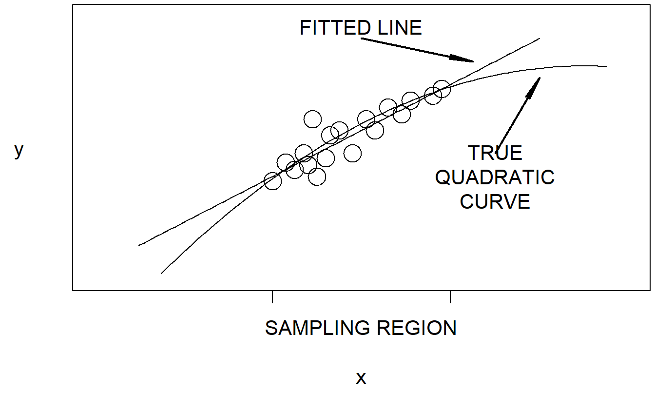
Figure 6.1: Extrapolation outside of the sampling region may be biased
Another pitfall due to a limited sampling region, although not a bias, that can arise is the difficulty in estimating a regression coefficient. In Chapter 5, we saw that a smaller spread of a variable, other things equal, means a less reliable estimate of the slope coefficient associated with that variable. That is, from Section 5.5.2 or equation (6.1), we see that the smaller is the spread of \(x_{j}\), as measured by \(s_{x_{j}}\), the larger is the standard error of \(b_{j},se(b_{j})\). Taken to the extreme, where \(s_{x_{j}}=0\), we might have a situation such as illustrated in Figure 6.2. For the extreme situation illustrated in Figure 6.2, there is not enough variation in \(x\) to estimate the corresponding slope parameter.
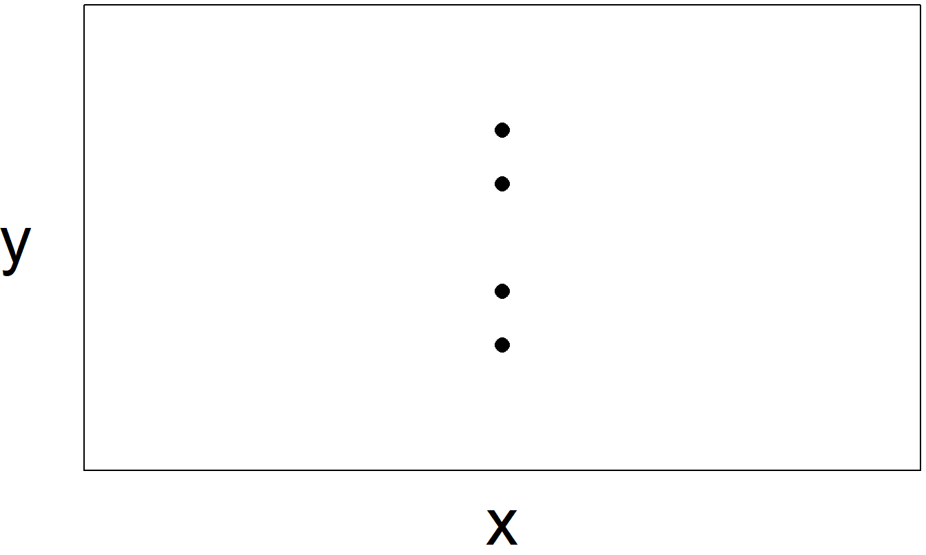
Figure 6.2: The lack of variation in \(x\) means that we cannot fit a unique line relating \(x\) and \(y\).
6.3.3 Limited Dependent Variables, Censoring and Truncation
In some applications, the dependent variable is constrained to fall within certain regions. To see why this is a problem, first recall that under the linear regression model, the dependent variable equals the regression function plus a random error. Typically, the random error is assumed to be approximately normally distributed, so that the response varies continuously. However, if the outcomes of the dependent variable are restricted, or limited, then the outcomes are not purely continuous. This means that our assumption of normal errors is not strictly correct, and may not even be a good approximation.
To illustrate, Figure 6.3 shows a plot of individual’s income (\(x\)) versus amount of insurance purchased (\(y\)). The sample in this plot represents two subsamples, those who purchased insurance, corresponding to \(y>0\), and those who did not, corresponding to “price” \(y=0\). Fitting a single line to these data would misinform users about the effects of \(x\) on \(y\).
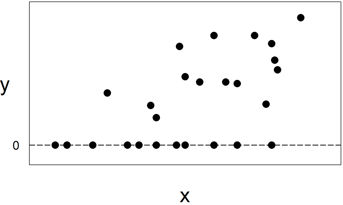
Figure 6.3: When individuals do not purchase anything, they are recorded as \(y=0\) sales.
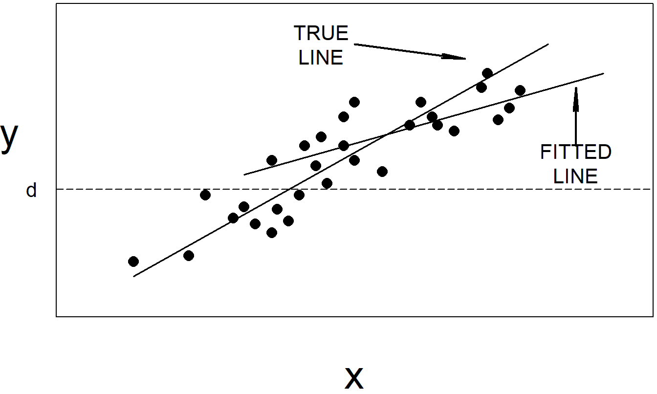
Figure 6.4: If the responses below the horizontal line at \(y=d\) are omitted, then the fitted regression line can be very different from the true regression line.
If we dealt with only those who purchased insurance then we still would have an implicit lower bound of zero (if an insurance price must exceed zero). However, prices need be close to this bound for a given sampling region and thus not represent an important practical problem. By including several individuals who did not purchase insurance (and thus spent $0 on insurance), our sampling region now clearly includes this lower bound.
There are several ways in which dependent variables can be restricted, or censored. Figure 6.3 illustrates the case in which the value of \(y\) may be no lower than zero. As another example, insurance claims are often restricted to be less than or equal to an upper limit specified in the insurance policy. If censoring is severe, ordinary least squares produces biased results. Specialized approaches, known as censored regression models, are described in Chapter 15 to handle this problem.
Figure 6.4 illustrates another commonly encountered limitation on the value of the dependent variable. For this illustration, suppose that \(y\) represents an insured loss and that \(d\) represents the deductible on an insurance policy. In this scenario, it is common practice for insurers to not record losses below \(d\) (they are typically not reported by policyholders). In this case, the data are said to be truncated. Not surprisingly, truncated regression models are available to handle this situation. As a rule of thumb, truncated data represent a more serious source of bias than censored data. When data are truncated, we do not have values of dependent variables and thus have less information than when the data are censored. See Chapter 15 for further discussion.
Video: Summary
6.3.4 Omitted and Endogenous Variables
Of course, analysts prefer to include all important variables. However, a common problem is that we may not have the resources nor the foresight to gather and analyze all the relevant data. Further, sometimes we are prohibited from including variables. For example, in insurance rating we are typically precluded from using ethnicity as a rating variable. Further, there are many mortality and other decrement tables that are “uni-sex,” that is, blind to gender.
Omitting important variables can affect our ability to fit the regression function; this can affect in-sample (explanation) as well as out-of-sample (prediction) performance. If the omitted variable is uncorrelated with other explanatory variables, then the omission will not affect estimation of regression coefficients. Typically this is not the case. The Section 3.4.3 Refrigerator Example illustrates a serious case where the direction of a statistically significant result was reversed based on the presence of an explanatory variable. In this example, we found that a cross-section of refrigerators displayed a significantly positive correlation between price and the annual energy cost of operating the refrigerator. This positive correlation was counter-intuitive because we would hope that higher prices would mean lower annual expenditures in operating a refrigerator. However, when we included several additional variables, in particular, measures of the size of a refrigerator, we found a significantly negative relationship between price and energy costs. Again, by omitting these additional variables, there was an important bias when using regression to understand the relationship between price and energy costs.
Omitted variables can lead to the presence of endogenous explanatory variables. An exogenous variable is one that can be taken as “given” for the purposes at hand. An endogenous variable is one that fails the exogeneity requirement. An omitted variable can affect both the \(y\) and the \(x\) and in this sense induce a relationship between the two variables. If the relationship between \(x\) and \(y\) is due to an omitted variable, it is difficult to condition on the \(x\) when estimating a model for \(y\).
Up to now, the explanatory variables have been treated as non-stochastic. For many social science applications, it is more intuitive to consider the \(x\)’s to be stochastic, and perform inference conditional on their realizations. For example, under common sampling schemes, we can estimate the conditional regression function \[ \mathrm{E~}\left(y|x_1, \ldots, x_k \right) = \beta_0 + \beta_1 x_1 + \ldots + \beta_k x_k . \] This is known as a “sampling-based” model.
In the economics literature, Goldberger (1972) defines a structural model as a stochastic model representing a causal relationship, not a relationship that simply captures statistical associations. Structural models can readily contain endogenous explanatory variables. To illustrate, we consider an example relating claims and premiums. For many lines of business, premium classes are simply nonlinear functions of exogenous factors such as age, gender and so forth. For other lines of business, premiums charged are a function of prior claims history. Consider model equations that relate one’s claims (\(y_{it}, t=1, 2\)) to premiums (\(x_{it}, t=1, 2\)): \[\begin{eqnarray*} y_{i2} = \beta_{0,C} + \beta_{1,C} y_{i1} + \beta_{2,C} x_{i2} + \varepsilon_{i1} \\ x_{i2} = \beta_{0,P} + \beta_{1,P} y_{i1} + \beta_{2,P} x_{i1} +\varepsilon_{i2} . \end{eqnarray*}\] In this model, current period (\(t=2\)) claims and premiums are affected by the prior period’s claims and premiums. This is an example of a structural equations model that requires special estimation techniques. Our usual estimation procedures are biased!
Example: Race, Redlining and Automobile Insurance Prices - Continued. Although Harrington and Niehaus (1998) did not find racial discrimination in insurance pricing, their results on access to insurance were inconclusive. Insurers offer “standard” and “preferred” risk contracts to applicants that meet restrictive underwriting standards, as compared to “substandard” risk contracts where underwriting standards are more relaxed. Expected claims are lower for standard and preferred risk contracts, and so premiums are lower, than substandard contracts. Harrington and Niehaus examined the proportion of applicants offered substandard contracts, NSSHARE, and found it significantly positively related to PCTBLACK, the proportion of population black. This suggests evidence of racial discrimination; they state this to be an inappropriate interpretation due to omitted variable bias.
Harrington and Niehaus argue that the proportion of applicants offered substandard contracts should be positively related to expected claim costs. Further, expected claim costs are strongly related to PCTBLACK, because minorities in the sample tended to be lower income. Thus, unobserved variables such as income tend to drive the positive relationship between NSSHARE and PCTBLACK. Because the data are analyzed at the zip code level and not at the individual level, the potential omitted variable bias rendered the analysis inconclusive.
6.3.5 Missing Data
In the data examples, illustrations, case studies and exercises of this text, there are many instances where certain data are unavailable for analysis, or missing. In every instance, the data were not carelessly lost but were unavailable due to substantive reasons associated with the data collection. For example, when we examined stock returns from a cross-section of companies, we saw that some companies did not have an average five year earnings per share figure. The reason was simply that they had not been in existence for five years. As another example, when examining life expectancies, some countries did not report the total fertility rate because they lacked administrative resources to capture this data. Missing data are an inescapable aspect of analyzing data in the social sciences.
When the reason for the lack of availability of data is unrelated to actual data values, the data are said to be missing at random. There are a variety of techniques for handling missing at random data, none of which are clearly superior to the others. One “technique” is to simply ignore the problem. Hence, missing at random is sometimes called the ignorable case of missing data.
If there are only a few missing data, compared to the total number available, a widely employed strategy is to delete the observations corresponding to the missing data. Assuming that the data are missing at random, little information is lost by deleting a small portion of the data. Further, with this strategy, we need not make additional assumptions about the relationships among the data.
If the missing data are primarily from one variable, we can consider omitting this variable. Here, the motivation is that we lose less information when omitting this variable as compared to retaining the variable but losing the observations associated with the missing data.
Another strategy is to fill in, or impute, missing data. There are many variations of the imputation strategy. All assume some type of relationships among the variables in addition to the regression model assumptions. Although these methods yield reasonable results, note that any type of filled-in values do not yield the same inherent variability as the real data. Thus, results of analyses based on imputed values often reflect less variability than those with real data.
Example: Insurance Company Expenses - Continued. When examining company financial information, analysts commonly are forced to omit substantial amounts of information when using regression models to search for relationships. To illustrate, Segal (2002) examined life insurance financial statements from data provided by the National Association of Insurance Commissioners (NAIC). He initially considered 733 firm-year observations over the period 1995-1998. However, 154 observations were excluded because of inconsistent or negative premiums, benefits and other important explanatory variables. Small companies representing 131 observations were also excluded. Small companies consist of fewer than 10 employees and agents, operating costs less than $1 million or fewer than 1,000 life policies sold. The resulting sample was \(n=448\) observations. The sample restrictions were based on explanatory variables - this procedure does not necessarily bias results. Segal argued that his final sample remained representative of the population of interest. There were about 110 firms in each of 1995-1998. In 1998, aggregate assets of the firms in the sample represent approximately $650 billion, a third of the life insurance industry.
Video: Section Summary
6.4 Missing Data Models
To understand the mechanisms that lead to unplanned nonresponse, we model it stochastically. Let \(r_i\) be a binary variable for the \(i\)th observation, with a one indicating that this response is observed and a zero indicating that the response is missing. Let \(\mathbf{r} = (r_1, \ldots, r_n)^{\prime}\) summarize the data availability for all subjects. The interest is in whether or not the responses influence the missing data mechanism. For notation, we use \(\mathbf{Y} = (y_1, \ldots, y_n)^{\prime}\) to be the collection of all potentially observed responses.
6.4.1 Missing at Random
In the case where \(\mathbf{Y}\) does not affect the distribution of \(\mathbf{r}\), we follow Rubin (1976) and call this case missing completely at random (MCAR). Specifically, the missing data are MCAR if \(\mathrm{f}(\mathbf{r} | \mathbf{Y}) = \mathrm{f}(\mathbf{r})\), where f(.) is a generic probability mass function. An extension of this idea is in Little (1995), where the adjective “covariate dependent” is added when \(\mathbf{Y}\) does not affect the distribution of \(\mathbf{r}\), conditional on the covariates. If the covariates are summarized as \(\mathbf{X}\), then the condition corresponds to the relation \(\mathrm{f}(\mathbf{r} | \mathbf{Y, X}) = \mathrm{f}(\mathbf{r | X})\). To illustrate this point, consider an example of Little and Rubin (1987) where \(\mathbf{X}\) corresponds to age and \(\mathbf{Y}\) corresponds to income of all potential observations. If the probability of being missing does not depend on income, then the missing data are MCAR. If the probability of being missing varies by age but does not by income over observations within an age group, then the missing data are covariate dependent MCAR. Under the latter specification, it is possible for the missing data to vary by income. For example, younger people may be less likely to respond to a survey. This shows that the “missing at random” feature depends on the purpose of the analysis. Specifically, it is possible that an analysis of the joint effects of age and income may encounter serious patterns of missing data whereas an analysis of income controlled for age suffers no serious bias patterns.
Little and Rubin (1987) advocate modeling the missing data mechanisms. To illustrate, consider a likelihood approach using a selection model for the missing data mechanism. Now, partition \(\mathbf{Y}\) into observed and missing components using the notation \(\mathbf{Y} =\{\mathbf{Y}_{obs}, \mathbf{Y}_{miss}\}\). With the likelihood approach, we base inference on the observed random variables. Thus, we use a likelihood proportional to the joint function \(\mathrm{f}(\mathbf{r}, \mathbf{Y}_{obs})\). We also specify a selection model by specifying the conditional mass function \(\mathrm{f}(\mathbf{r} | \mathbf{Y})\).
Suppose that the observed responses and the selection model distributions are characterized by vectors of parameters \(\boldsymbol \theta\) and \(\boldsymbol \psi\) , respectively. Then, with the relation \(\mathrm{f}(\mathbf{r}, \mathbf{Y}_{obs},\boldsymbol \theta, \boldsymbol \psi)\) \(= \mathrm{f}(\mathbf{Y}_{obs}, \boldsymbol \theta) \times \mathrm{f}(\mathbf{r} | \mathbf{Y}_{obs}, \boldsymbol \psi)\), we may express the log likelihood of the observed random variables as
\[ L(\boldsymbol \theta, \boldsymbol \psi) = \mathrm{ln~} \mathrm{f}(\mathbf{r}, \mathbf{Y}_{obs}, \boldsymbol \theta, \boldsymbol \psi) = \mathrm{ln~} \mathrm{f}(\mathbf{Y}_{obs}, \boldsymbol \theta) + \mathrm{ln~} \mathrm{f}(\mathbf{r} | \mathbf{Y}_{obs}, \boldsymbol \psi). \] (See Section 11.9 if you would like a refresher on likelihood inference.) In the case where the data are MCAR, then \(\mathrm{f}(\mathbf{r} | \mathbf{Y}_{obs}, \boldsymbol \psi) = \mathrm{f}(\mathbf{r} | \boldsymbol \psi)\) does not depend on \(\mathbf{Y}_{obs}\). Little and Rubin (1987) also consider the case where the selection mechanism model distribution does not depend on \(\mathbf{Y}_{miss}\) but may depend on \(\mathbf{Y}_{obs}\). In this case, they call the data missing at random (MAR).
In both the MAR and MCAR cases, we see that the likelihood may be maximized over the parameters, separately for each case. In particular, if one is only interested in the maximum likelihood estimator of \(\boldsymbol \theta\), then the selection model mechanism may be “ignored.” Hence, both situations are often referred to as the ignorable case.
Example: Dental Expenditures. Let \(y\) represent a household’s annual dental expenditure and \(x\) represent income. Consider the following five selection mechanisms.
- The household is not selected (missing) with probability without regard to the level of dental expenditure. In this case, the selection mechanism is MCAR.
- The household is not selected if the dental expenditure is less than $100. In this case, the selection mechanism depends on the observed and missing response. The selection mechanism cannot be ignored.
- The household is not selected if the income is less than $20,000. In this case, the selection mechanism is MCAR, covariate dependent. That is, assuming that the purpose of the analysis is to understand dental expenditures conditional on knowledge of income, stratifying based on income does not seriously bias the analysis.
- The probability of a household being selected increases with dental expenditure. For example, suppose the probability of being selected is a linear function of \(\exp(\psi y_i)/(1+ \exp(\psi y_i))\). In this case, the selection mechanism depends on the observed and missing response. The selection mechanism cannot be ignored.
- The household is followed over \(T\) = 2 periods. In the second period, a household is not selected if the first period expenditure is less than $100. In this case, the selection mechanism is MAR. That is, the selection mechanism is based on an observed response.
The second and fourth selection mechanisms represent situations where the selection mechanism must be explicitly modeled; these are non-ignorable cases. In these situations without explicit adjustments, procedures that ignore the selection effect may produce seriously biased results. To illustrate a correction for selection bias in a simple case, we outline an example due to Little and Rubin (1987). Section 6.4.2 describes additional mechanisms.
Example: Historical Heights. Little and Rubin (1987) discuss data due to Wachter and Trusell (1982) on \(y\), the height of men recruited to serve in the military. The sample is subject to censoring in that minimum height standards were imposed for admission to the military. Thus, the selection mechanism is \[ r_i = \left\{ \begin{array}{ll} 1 & y_i > c_i \\ 0 & \mathrm{otherwise} \\ \end{array} \right. , \] where \(c_i\) is the known minimum height standard imposed at the time of recruitment. The selection mechanism is non-ignorable because it depends on the individual’s height, \(y\).
For this example, additional information is available to provide reliable model inference. Specifically, based on other studies of male heights, we may assume that the population of heights is normally distributed. Thus, the likelihood of the observables can be written down and inference may proceed directly. To illustrate, suppose that \(c_i = c\) is constant. Let \(\mu\) and \(\sigma\) denote the mean and standard deviation of \(y\). Further suppose that we have a random sample of \(n + m\) men in which \(m\) men fall below the minimum standard height \(c\) and we observe \(\mathbf{Y}_{obs} = (y_1, \ldots, y_n)^{\prime}\). The joint distribution for observables is
\[\begin{eqnarray*} \mathrm{f}(\mathbf{r}, \mathbf{Y}_{obs}, \mu, \sigma) &=& \mathrm{f}(\mathbf{Y}_{obs}, \mu, \sigma) \times \mathrm{f}(\mathbf{r} | \mathbf{Y}_{obs}) \\ &=& \left\{ \prod_{i=1}^n \mathrm{f}(y_i | y_i > c) \times \mathrm{Pr}(y_i > c) \right\} \times \left\{\mathrm{Pr}(y_i \leq c)\right\}^m. \end{eqnarray*}\] Now, let \(\phi\) and \(\Phi\) represent the density and distribution function for the standard normal distribution. Thus, the log-likelihood is \[\begin{eqnarray*} L(\mu, \sigma) &=& \mathrm{ln~} \mathrm{f}(\mathbf{r}, \mathbf{Y}_{obs}, \mu, \sigma) \\ &=& \sum_{i=1}^n \mathrm{ln}\left\{ \frac{1}{\sigma} \phi \left( \frac{y_i-\mu}{\sigma} \right) \right\} + m~ \mathrm{ln}\left\{ \Phi \left( \frac{c-\mu}{\sigma}\right) \right\} . \end{eqnarray*}\] This is easy to maximize in \(\mu\) and \(\sigma\). If one ignored the censoring mechanisms, then one would derive estimates of the observed data from the “log likelihood,” \[ \sum_{i=1}^n \mathrm{ln}\left\{ \frac{1}{\sigma} \phi \left( \frac{y_i-\mu}{\sigma} \right) \right\}, \] yielding different, and biased, results.
6.4.2 Non-Ignorable Missing Data
For non-ignorable missing data, Little (1995) recommends:
- Avoid missing responses whenever possible by using appropriate follow-up procedures.
- Collect covariates that are useful for predicting missing values.
- Collect as much information as possible regarding the nature of the missing data mechanism.
For the last point, if little is known about the missing data mechanism, then it is difficult to employ a robust statistical procedure to correct for the selection bias.
There are many models of missing data mechanisms. A general overview appears in Little and Rubin (1987). Little (1995) surveys the problem of attrition. Rather than survey this developing literature, we give a widely used model of non-ignorable missing data.
Heckman Two-Stage Procedure
Heckman (1976) assumes that the sampling response mechanism is governed by the latent (unobserved) variable \(r_i^{\ast}\) where \[ r_i^{\ast} = \mathbf{z}_i^{\prime} \boldsymbol \gamma + \eta_i. \] The variables in \(\mathbf{z}_i\) may or may not include the variables in \(\mathbf{x}_i\). We observe \(y_i\) if \(r_i^{\ast}>0\), that is, if \(r_i^{\ast}\) crosses the threshold 0. Thus, we observe \[ r_i = \left\{ \begin{array}{ll} 1 & r_i^{\ast}>0 \\ 0 & \mathrm{otherwise} \\ \end{array} \right. . \] To complete the specification, we assume that {(\(\varepsilon_i,\eta_i\))} are identically and independently distributed, and that the joint distribution of (\(\varepsilon_i,\eta_i\)) is bivariate normal with means zero, variances \(\sigma^2\) and \(\sigma_{\eta}^2\) and correlation \(\rho\). Note that if the correlation parameter \(\rho\) equals zero, then the response and selection models are independent. In this case, the data are MCAR and the usual estimation procedures are unbiased and asymptotically efficient.
Under these assumptions, basic multivariate normal calculations show that \[ \mathrm{E~}(y_i | r_i^{\ast}>0) = \mathbf{x}_i^{\prime} \boldsymbol \beta + \beta_{\lambda} \lambda(\mathbf{z}_i^{\prime} \boldsymbol \gamma), \] where \(\beta_{\lambda} = \rho \sigma\) and \(\lambda(a)=\phi(a)/\Phi(a)\). Here, \(\lambda(.)\) is the inverse of the so-called “Mills ratio.” This calculation suggests the following two-step procedure for estimating the parameters of interest.
Heckman’s Two-Stage Procedure
- Use the data {(\(r_i, \mathbf{z}_i\))} and a probit regression model to estimate \(\boldsymbol \gamma\). Call this estimator \(\mathbf{g}_H\).
- Use the estimator from stage (1) to create a new explanatory variable, \(x_{i,K+1} = \lambda(\mathbf{z}_i^{\prime}\mathbf{g}_H)\). Run a regression model using the \(K\) explanatory variables \(\mathbf{x}_i\) as well as the additional explanatory variable \(x_{i,K+1}\). Use \(\mathbf{b}_H\) and \(b_{\lambda,H}\) to denote the estimators of \(\boldsymbol \beta\) and \(\beta_{\lambda}\), respectively.
Chapter 11 will introduce probit regressions. We also note that the two-step method does not work in absence of covariates to predict the response and, for practical purposes, requires variables in \(\mathbf{z}\) that are not in \(\mathbf{x}\) (see Little and Rubin, 1987).
To test for selection bias, we may test the null hypothesis \(H_0:\beta_{\lambda}=0\) in the second stage due to the relation \(\beta_{\lambda}= \rho \sigma\). When conducting this test, one should use heteroscedasticity-corrected standard errors. This is because the conditional variance \(\mathrm{Var}(y_i | r_i^{\ast}>0)\) depends on the observation \(i\). Specifically, \(\mathrm{Var}(y_i | r_i^{\ast}>0) = \sigma^2 (1-\rho^2 \delta_i),\) where \(\delta_i= \lambda_i(\lambda_i + \mathbf{z}_i^{\prime} \boldsymbol \gamma)\) and \(\lambda_i = \phi(\mathbf{z}_i^{\prime} \boldsymbol \gamma)/\Phi(\mathbf{z}_i^{\prime} \boldsymbol \gamma).\)
This procedure assumes normality for the selection latent variables to form the augmented variables. Other distribution forms are available in the literature, including the logistic and uniform distributions. A deeper criticism, raised by Little (1985), is that the procedure relies heavily on assumptions that cannot be tested using the data available. This criticism is analogous to the historical heights example where we relied heavily on the normal curve to infer the distribution of heights below the censoring point. Despite these criticisms, Heckman’s procedure is widely used in the social sciences.
EM algorithm
Section 6.4.2 has focused on introducing specific models of non-ignorable nonresponse. General robust models of nonresponse are not available. Rather, a more appropriate strategy is to focus on a specific situation, collect as much information as possible regarding the nature of the selection problem and then develop a model for this specific selection problem.
The EM algorithm is a computational device for computing model parameters. Although specific to each model, it has found applications in a wide variety of models involving missing data. Computationally, the algorithm iterates between the “E,” for conditional expectation, and “M,” for maximization, steps. The E step finds the conditional expectation of the missing data given the observed data and current values of the estimated parameters. This is analogous to the time-honored tradition of imputing missing data. A key innovation of the EM algorithm is that one imputes sufficient statistics for missing values, not the individual data points. For the M step, one updates parameter estimates by maximizing an observed log likelihood. Both the sufficient statistics and the log likelihood depend on the model specification.
Many introductions of the EM algorithm are available in the literature. Little and Rubin (1987) provide a detailed treatment.
6.5 Application: Risk Managers’ Cost Effectiveness
This section examines data from a survey on the cost effectiveness of risk management practices. Risk management practices are activities undertaken by a firm to minimize the potential cost of future losses, such as the event of a fire in a warehouse or an accident that injures employees. This section develops a model that can be used to make statements about cost of managing risks.
An outline of the regression modeling process is as follows. We begin by providing an introduction to the problem and giving some brief background on the data. Certain prior theories will lead us to present a preliminary model fit. Using diagnostic techniques, it will be evident that several assumptions underpinning this model are not in accord with the data. This will lead us to go back to the beginning and start the analysis from scratch. Things that we learn from a detailed examination of the data will lead us to postulate some revised models. Finally, to communicate certain aspects of the new model, we will explore graphical presentations of the recommended model.
Introduction
The data for this study were provided by Professor Joan Schmit and are discussed in more detail in the paper, “Cost effectiveness of risk management practices,” Schmit and Roth (1990). The data are from a questionnaire that was sent to 374 risk managers of large U.S.-based organizations. The purpose of the study was to relate cost effectiveness to management’s philosophy of controlling the company’s exposure to various property and casualty losses, after adjusting for company effects such as size and industry type.
First, some caveats. Survey data are often based on samples of convenience, not probability samples. Just as with all observational data sets, regression methodology is a useful tool for summarizing data. However, we must be careful when making inferences based on this type of data set. For this particular survey, 162 managers returned completed surveys resulting in a good response rate of \(43\%\). However, for the variables included in the analysis (defined below), only 73 forms were completed resulting in a complete response rate of \(20\%\). Why such a dramatic difference? Managers, like most people, typically do not mind responding to queries about their attitudes, or opinions, about various issues. When questioned about hard facts, in this case company asset size or insurance premiums, either they considered the information proprietary and were reluctant to respond even when guaranteed anonymity or they simply were not willing to take the time to look up the information. From a surveyor’s standpoint, this is unfortunate because typically “attitudinal” data are fuzzy (high variance compared to the mean) as compared to hard financial data. The tradeoff is that the latter data are often hard to obtain. In fact, for this survey, several pre-questionnaires were sent to ascertain managers’ willingness to answer specific questions. From the pre-questionnaires, the researchers severely reduced the number of financial questions that they intended to ask.
A measure of risk management cost effectiveness, FIRMCOST, is the dependent variable. This variable is defined as total property and casualty premiums and uninsured losses as a percentage of total assets. It is a proxy for annual expenditures associated with insurable events, standardized by company size. Here, for the financial variables, ASSUME is the per occurrence retention amount as a percentage of total assets, CAP indicates whether the company owns a captive insurance company, SIZELOG is the logarithm of total assets and INDCOST is a measure of the firm’s industry risk. Attitudinal variables include CENTRAL, a measure of the importance of the local managers in choosing the amount of risk to be retained and SOPH, a measure of the degree of importance in using analytical tools, such as regression, in making risk management decisions.
In the paper, the researchers described several weaknesses of the definitions used but argue that these definitions provide useful information, based on the willingness of risk managers to obtain reliable information. The researchers also described several theories concerning relationships that may be confirmed by the data. Specifically, they hypothesized:
- There exists an inverse relationship between the risk retention (ASSUME) and cost (FIRMCOST). The idea behind this theory is that larger retention amounts should mean lower expenses to a firm, resulting in lower costs.
- The use of a captive insurance company (CAP) results in lower costs. Presumably, a captive is used only when cost effective and consequently, this variable should indicate lower costs if used effectively.
- There exists an inverse relationship between the measure of centralization (CENTRAL) and cost (FIRMCOST). Presumably, local managers would be able to make more cost-effective decisions because they are more familiar with local circumstances regarding risk management than centrally located managers.
- There exists an inverse relationship between the measure of sophistication (SOPH) and cost (FIRMCOST). Presumably, more sophisticated analytical tools help firms to manage risk better, resulting in lower costs.
Preliminary Analysis
To test the theories described above, the regression analysis framework can be used. To do this, posit the model
\[ \small{ \begin{array}{ll} \text{FIRMCOST} &=&\beta_0 +\beta_1 \text{ ASSUME}+\beta_{2}\text{ CAP} +\beta_{3}\text{ SIZELOG}+\beta_4\text{ INDCOST} \\ &&+\beta_5\text{ CENTRAL}+\beta_6\text{ SOPH}+ \varepsilon. \end{array} } \]
With this model, each theory can be interpreted in terms of regression coefficients. For example, \(\beta_1\) can be interpreted as the expected change in cost per unit change in retention level (ASSUME). Thus, if the first hypothesis is true, we expect \(\beta_1\) to be negative. To test this, we can estimate \(b_{1}\) and use our tests of hypotheses machinery to decide if \(b_{1}\) is significantly less than zero. The variables SIZELOG and INDCOST are included in the model to control for the effects of these variables. These variables are not directly under a risk manager’s control and thus are not of primary interest. However, inclusion of these variables can account for an important part of the variability.
Data from 73 managers was fit using this regression model. Table 6.2 summarizes the fitted model.
| Coefficient | Standard Error | \(t\)-Statistic | |
|---|---|---|---|
| (Intercept) | 59.765 | 19.065 | 3.135 |
| ASSUME | -0.300 | 0.222 | -1.353 |
| CAP | 5.498 | 3.848 | 1.429 |
| SIZELOG | -6.836 | 1.923 | -3.555 |
| INDCOST | 23.078 | 8.304 | 2.779 |
| CENTRAL | 0.133 | 1.441 | 0.092 |
| SOPH | -0.137 | 0.347 | -0.394 |
The adjusted coefficient of determination is \(R_{a}^{2}=18.8\%\), the \(F\)-ratio is 3.78 and the residual standard deviation is \(s=14.56\).
On the basis of the summary statistics from the regression model, we can conclude that the measures of centralization and sophistication do not have an impact on our measure of cost effectiveness. For both of these variables the \(t\)-ratio is low, less than 1.0 in absolute value. The effect of risk retention seems only somewhat important. The coefficient has the appropriate sign although is only 1.35 standard errors below zero. This would not be considered statistically significant at the 5% level, although it would be at the 10% level (the \(p\)-value is 9%). Perhaps most perplexing is the coefficient associated with the CAP variable. We theorized that this coefficient would be negative. However, in our analysis of the data, the coefficient turns out to be positive and is 1.43 standard errors above zero. This not only leads us to disaffirm our theory, but also to search for new ideas that are in accord with the information learned from the data. Schmit and Roth suggest reasons that may help us interpret the results of our hypothesis testing procedures. For example, they suggest that managers in the sample may not have the most sophisticated tools available to them when managing risks, resulting in an insignificant coefficient associated with SOPH. They also discussed alternative suggestions, as well as interpretations for the other results of the tests of hypotheses.
How robust is this model? Section 6.2 emphasized some of the dangers of working with an inadequate model. Some readers may feel uncomfortable with the model selected above because two out of the six variables have \(t\)-ratios less than 1 in absolute value and four out of six have \(t\)-ratios less than 1.5 in absolute value. Perhaps even more important, histograms of the standardized residuals and leverages, in Figure 6.5, show several observations to be outliers and high leverage points. To illustrate, the largest residual turns out to be \(e_{15}=83.73\). The error sum of squares is \(Error~SS\) = \((n-(k+1))s^{2}\) = \((73-7)(14.56)^{2}=13,987\). Thus, the 15th observation represents 50.1% of the error sum of squares \((=83.73^{2}/13,987)\), suggesting that this 1 observation out of 73 has a dominant impact on the model fit. Further, plots of standardized residuals versus fitted values, not presented here, displayed evidence of heteroscedastic residuals. Based on these observations, it seems reasonable to assess the robustness of the model.
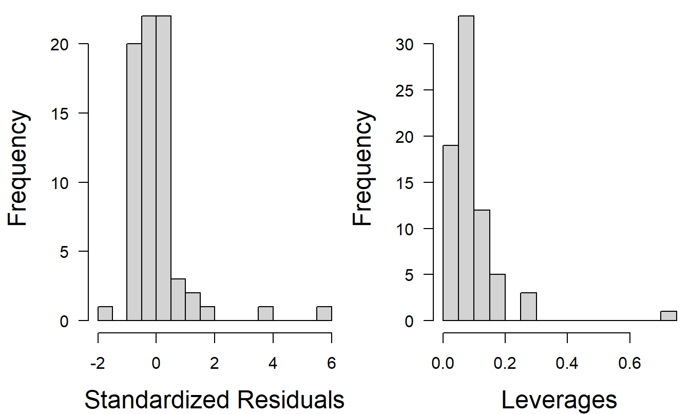
Figure 6.5: Histograms of standardized residuals and leverages from a preliminary regression model fit.
R Code to Produce Table 6.2 and Figure 6.5
Back to the Basics
To get a better understanding of the data, we begin by examining the basic summary statistics in Table 6.3 and corresponding histograms in Figure 6.6. From Table 6.3, the largest value of FIRMCOST is 97.55, which is more than five standard deviations above the mean \([10.97+5(16.16)=91.77]\). An examination of the data shows that this point is observation 15, the same observation that was an outlier in the preliminary regression fit. However, the histogram of FIRMCOST in Figure 6.6 reveals that this is not the only unusual point. Two other observations have unusually large values of FIRMCOST, resulting in a distribution that is skewed to the right. The histogram, in Figure 6.6, of the ASSUME variable shows that this distribution is also skewed to the right, possibly due solely to two large observations. From the basic summary statistics in Table 6.3, we see that the largest value of ASSUME is more than seven standard deviations above the mean. This observation may well turn out to be influential in subsequent regression model fitting. The scatterplot of FIRMCOST versus ASSUME in Figure 6.6 tells us that the observation with the largest value of FIRMCOST is not the same as the observation with the largest value of ASSUME.
| Mean | Median | Standard Deviation | Minimum | Maximum | |
|---|---|---|---|---|---|
| FIRMCOST | 10.973 | 6.08 | 16.159 | 0.20 | 97.55 |
| ASSUME | 2.574 | 0.51 | 8.445 | 0.00 | 61.82 |
| CAP | 0.342 | 0.00 | 0.478 | 0.00 | 1.00 |
| SIZELOG | 8.332 | 8.27 | 0.963 | 5.27 | 10.60 |
| INDCOST | 0.418 | 0.34 | 0.216 | 0.09 | 1.22 |
| CENTRAL | 2.247 | 2.00 | 1.256 | 1.00 | 5.00 |
| SOPH | 21.192 | 23.00 | 5.304 | 5.00 | 31.00 |
Source: Schmit and Roth, (1990)
From the histograms of SIZELOG, INDCOST, CENTRAL, and SOPH, we see that these distributions are not heavily skewed. Taking logarithms of the size of total company assets has served to make the distribution more symmetric than in the original units. From the histogram and summary statistics, we see that CENTRAL is a discrete variables, taking on values one through five. The other discrete variable is CAP, a binary variable taking values only zero and one. The histogram and scatter plot corresponding to CAP is not presented here. It is more informative to provide a table of means of each variable by levels of CAP, as in Table 6.4. From this table, we see that 25 of the 73 companies surveyed own captive insurers. Further, on one hand, the average FIRMCOST for those companies with captive insurers \((\)CAP \(=1)\) is larger than those without \((\)CAP \(=0)\). On the other hand, when moving to the logarithmic scale, the opposite is true; that is, average COSTLOG for those companies with captive insurers \((\)CAP \(=1)\) is larger than those without \((\)CAP \(=0)\).
| \(n\) | FIRMCOST | ASSUME | SIZELOG | INDCOST | CENTRAL | SOPH | COSTLOG | |
|---|---|---|---|---|---|---|---|---|
| CAP = 0 | 48 | 9.954 | 1.175 | 8.196 | 0.399 | 2.250 | 21.521 | 1.820 |
| CAP = 1 | 25 | 12.931 | 5.258 | 8.592 | 0.455 | 2.240 | 20.560 | 1.595 |
| TOTAL | 73 | 10.973 | 2.574 | 8.332 | 0.418 | 2.247 | 21.192 | 1.743 |
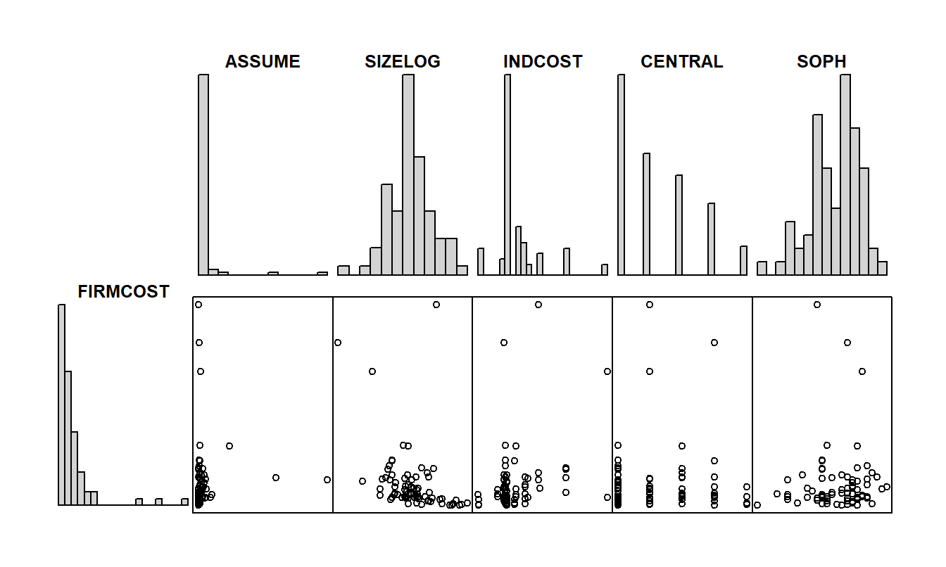
Figure 6.6: Histograms and scatter plots of FIRMCOST and several explanatory variables. The distributions of FIRMCOST and ASSUME are heavily skewed to the right. There is a negative relationship between FIRMCOST and SIZELOG, although nonlinear.
R Code to Produce Tables 6.3 and 6.4 and Figure 6.6
When examining relationships between pairs of variables, in Figure 6.6 we see some of the relationships that were evident from preliminary regression fit. There is an inverse relationship between FIRMCOST and SIZELOG, and the scatterplot plot suggests this relationship may be nonlinear. There is also a mild positive relationship between FIRMCOST and INDCOST and no apparent relationships between FIRMCOST and any of the other explanatory variables. These observations are reinforced by the table of correlations given in Table 6.4. Note that the table masks a feature that is evident in the scatter plots, the effect of the unusually large observations.
| COSTLOG | FIRMCOST | ASSUME | CAP | SIZELOG | INDCOST | CENTRAL | |
|---|---|---|---|---|---|---|---|
| FIRMCOST | 0.713 | ||||||
| ASSUME | 0.165 | 0.039 | |||||
| CAP | -0.088 | 0.088 | 0.231 | ||||
| SIZELOG | -0.637 | -0.366 | -0.209 | 0.196 | |||
| INDCOST | 0.395 | 0.326 | 0.249 | 0.122 | -0.102 | ||
| CENTRAL | -0.054 | 0.014 | -0.068 | -0.004 | -0.08 | -0.085 | |
| SOPH | 0.144 | 0.048 | 0.062 | -0.087 | -0.209 | 0.093 | 0.283 |
Because of the skewness of the distribution and the effect of the unusually large observations, a transformation of the response variable might lead to fruitful results. Figure 6.7 is the histogram of COSTLOG, defined to be the logarithm of FIRMCOST. The distribution is much less skewed than the distribution of FIRMCOST. The variable COSTLOG was also included in the correlation matrix in Table 6.4. From this table, the relationship between SIZELOG appears to be stronger with COSTLOG than with FIRMCOST. Figure 6.8 shows several scatter plots illustrating the relationship between COSTLOG and the explanatory variables. The relationship between COSTLOG and SIZELOG appears to be linear. It is easier to interpret these scatter plots than those in Figure 6.6 due to the absence of the large unusual values of the dependent variable.
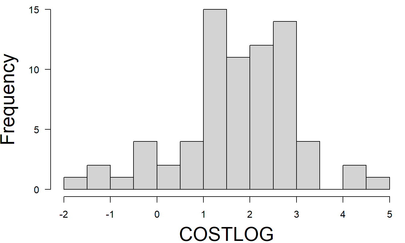
Figure 6.7: Histogram of COSTLOG (the natural logarithm of FIRMCOST). The distribution of COSTLOG is less skewed than that of FIRMCOST.
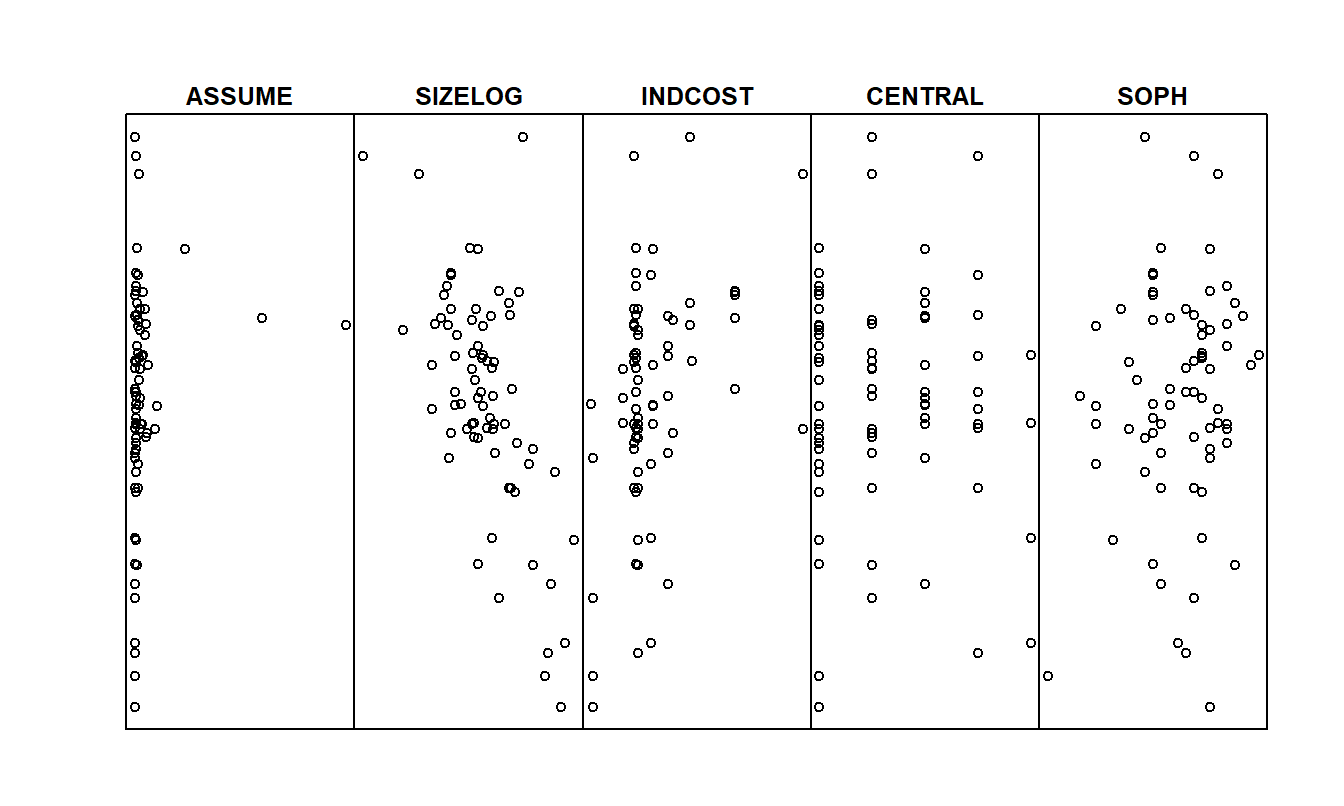
Figure 6.8: Scatter plots of COSTLOG versus several explanatory variables. There is a negative relationship between COSTLOG and SIZELOG and a mild positive relationship between COSTLOG and INDCOST.
R Code to Produce Table 6.5 and Figures 6.7 and 6.8
Some New Models
Now, we explore the use of COSTLOG as the dependent variable. This line of thought is based on the work in the previous subsection and the plots of residuals from the preliminary regression fit. As a first step, we fit a model with all explanatory variables. Thus, this model is the same as the preliminary regression fit except using COSTLOG in lieu of FIRMCOST as the dependent variable. This model serves as a useful benchmark for our subsequent work. Table 6.6 summarizes the fit.
| Coefficient | Standard Error | \(t\)-Statistic | |
|---|---|---|---|
| (Intercept) | 7.643 | 1.155 | 6.617 |
| ASSUME | -0.008 | 0.013 | -0.609 |
| CAP | 0.015 | 0.233 | 0.064 |
| SIZELOG | -0.787 | 0.116 | -6.752 |
| INDCOST | 1.905 | 0.503 | 3.787 |
| CENTRAL | -0.080 | 0.087 | -0.916 |
| SOPH | 0.002 | 0.021 | 0.116 |
Here, \(R_{a}^{2}=48\%\), \(F\)-ratio \(=12.1\) and \(s=0.882\). Figure 6.9 shows that the distribution of standardized residuals is less skewed than the corresponding in Figure 6.5. The distribution of leverages shows that there are still highly influential observations. (As a matter of fact, the distribution of leverages appear to be the same as in Figure 6.5. Why?) Four of the six variables have \(t\)-ratios less than one in absolute value, suggesting that we continue our search for a better model.
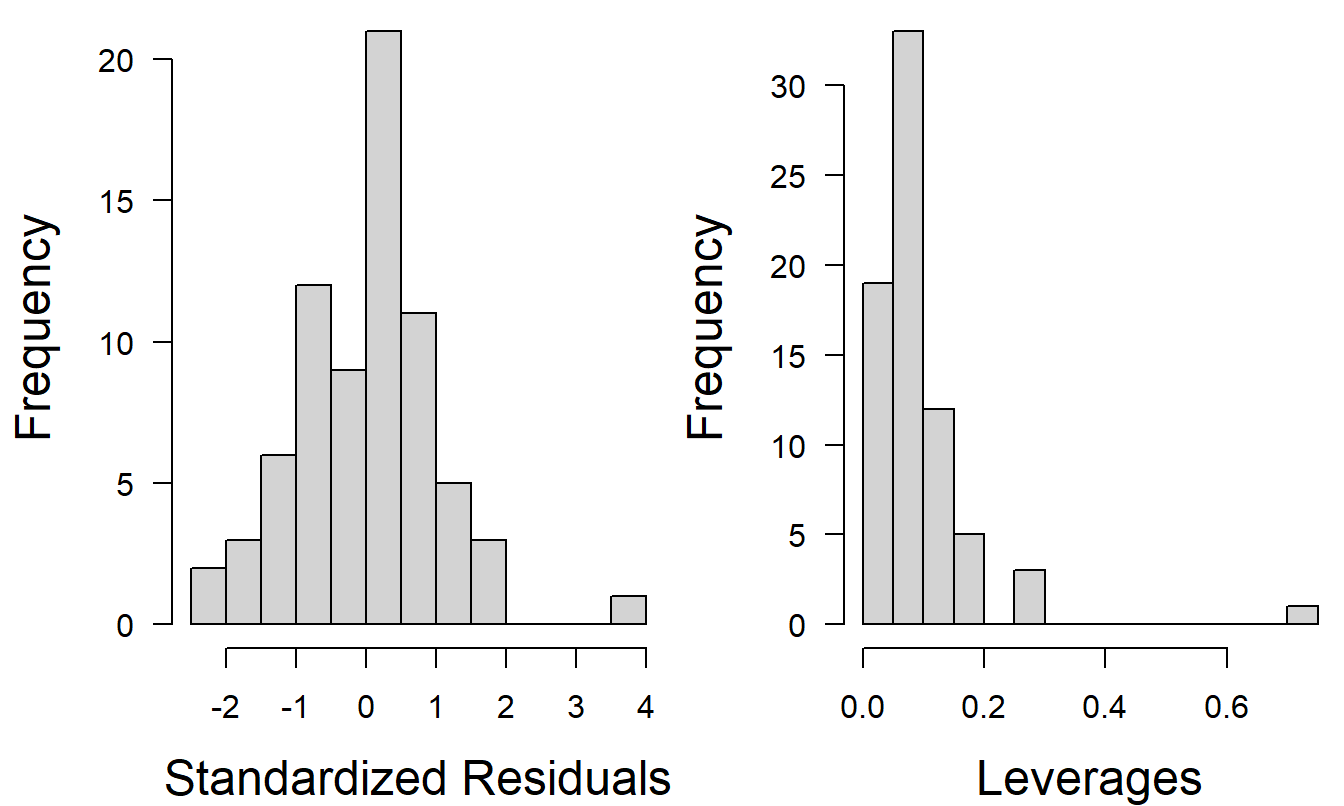
Figure 6.9: Histograms of standardized residuals and leverages using COSTLOG as the dependent variable.
To continue the search, a stepwise regression was run (although the output is not reproduced here). The output from this search technique, as well as the fitted regression model above, suggests using the variables SIZELOG and INDCOST to explain the dependent variable COSTLOG.
We can run regression using SIZELOG and INDCOST as explanatory variables. From Figure 6.10, we see that the size and shape of the distribution of standardized residuals are similar to that in Figure 6.9. The leverages are much smaller, reflecting the elimination of several explanatory variables from the model. Remember that the average leverage is \(\bar{h} =(k+1)/n=3/73\approx 0.04\). Thus, we still have three points that exceed three times the average and thus are considered high leverage points.
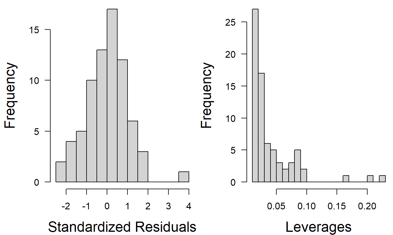
Figure 6.10: Histograms of standardized residuals and leverages using SIZELOG and INDCOST as explanatory variables.
R Code to Produce Table 6.6 and Figures 6.9 and 6.10
| Coefficient | Standard Error | \(t\)-Statistic | |
|---|---|---|---|
| (Intercept) | 6.353 | 0.953 | 6.666 |
| SIZELOG | -0.773 | 0.101 | -7.626 |
| INDCOST | 6.264 | 1.610 | 3.889 |
| INDCOSTSQ | -3.585 | 1.265 | -2.833 |
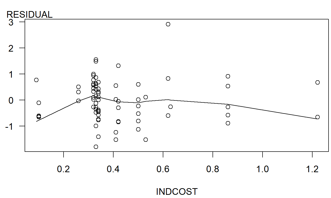
Figure 6.11: Scatter plot of residuals versus INDCOST. The smooth fitted curve (using lowess) suggests a quadratic term in INDCOST.
R Code to Produce Table 6.7 and Figure 6.11
Plots of residuals versus the explanatory variables reveal some mild patterns. The scatter plot of residuals versus INDCOST, in Figure 6.11, displays a mild quadratic trend in INDCOST. To see if this trend was important, the variable INDCOST was squared and used as an explanatory variable in a regression model. The results of this fit are in Table 6.6.
From the \(t\)-ratio associated with (INDCOST)\(^{2}\), we see that the variable seems to be important. The sign is reasonable, indicating that the rate of increase of COSTLOG decreases as INDCOST increases. That is, the expected change in COSTLOG per unit change of INDCOST is positive and decreases as INDCOST increases.
Further diagnostic checks of the model revealed no additional patterns. Thus, from the data available, we can not affirm any of the four hypotheses that were introduced in the Introduction subsection. This is not to say that these variables are not important. We are simply stating that the natural variability of the data was large enough to obscure any relationships that might exist. We have established, however, the importance of the size of the firm and the firm’s industry risk.
Figure 6.12 graphically summarizes the estimated relationships among these variables. In particular, in lower right hand panel, we see that for most of the firms in the sample, FIRMCOST was relatively stable. However, for small firms, as measured by SIZELOG, the industry risk, as measured by INDCOST, was particularly important. For small firms, we see that the fitted FIRMCOST increases as the variable INDCOST increases, with the rate of increase leveling off. Although the model theoretically predicts FIRMCOST to decrease with a large INDCOST \((>1.2)\), no small firms were actually in this area of the data region.
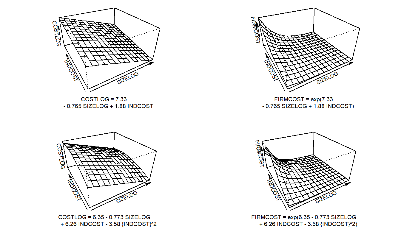
Figure 6.12: Graph of four fitted models versus INDCOST and SIZELOG.
6.6 Further Reading and References
This chapter concludes our Part I, an introduction to linear regression. To learn more about linear regression, in Section 1.7 we gave references to alternative statistics books that introduce the topic. You may also be interested in a more technical presentation, such as the classic work by Seber (1977) or a more recent work by Abraham and Ledolter (2006). For other approaches, texts such as Wooldridge (2009) provide an econometrics perspective where the emphasis is on introducing regression in the context of economic theory. Alternatively, books such as Agresti and Finlay (2008) give an introduction from a broader social science perspective.
There are many explanations of regression for readers with different perspectives and levels of quantitative training; this provides further evidence that this is an important topic for actuaries and other financial risk managers to understand. The other way of getting further insights into linear regression is to see it applied in a time series context in Part II of this book or in extensions to nonlinear modeling in Part III.
See Bollen (1989) for a classic introduction to structural equations modeling.
Chapter References
- Abraham, Bova and Johannes Ledolter (2006). Introduction to Regression Modeling. Thomson Higher Education, Belmont, CA.
- Agresti, Alan and Barbara Finlay (2008). Statistical Methods for the Social Sciences, Fourth Edition. Prentice Hall, Upper Saddle, NJ.
- Bollen, Kenneth A. (1989). Structural Equations with Latent Variables. New York: Wiley.
- Box, George E. P. (1979). Robustness in the strategy of scientific model building. In R. Launer and G. Wilderson (editors), Robustness in Statistics, pages 201-236, Academic Press, New York.
- Faraway, Julian J. (2005). Linear Models with R. Chapman & Hall/CRC, Boca Raton, Florida.
- Fienberg, S. E (1985). Insurance availability in Chicago. Chapter in Data: A Collection of Problems from Many Fields for the Student and Research Worker. Editors D.F. Andrews and A. M. Herzberg, Springer-Verlag, New York.
- Goldberger, Arthur S. (1972). Structural equation methods in the social sciences. Econometrica 40, 979-1001.
- Harrington, Scott E. and Greg Niehaus (1998). Race, redlining and automobile insurance prices. Journal of Business 71(3), 439-469.
- Heckman, J. J. (1976). The common structure of statistical models of truncation, sample selection and limited dependent variables, and a simple estimator for such models. Ann. Econ. Soc. Meas. 5, 475-492.
- Little, R. J. (1995). Modelling the drop-out mechanism in repeated-measures studies. Journal of the American Statistical Association 90, 1112-1121.
- Little, R. J. and Rubin, D. B. (1987). Statistical Analysis with Missing Data. John Wiley, New York.
- Roberts, Harry V. (1990). Business and economic statistics (with discussion). Statistical Science 4, 372-402.
- Rubin, D. R. (1976). Inference and missing data. Biometrika 63, 581-592.
- Schmit, Joan T. and K. Roth (1990). Cost effectiveness of risk management practices. The Journal of Risk and Insurance 57, No. 3, pages 455-470.
- Seber, G. A. F. (1977). Linear Regression Analysis. John Wiley & Sons, New York.
- Wachter, K. W. and J. Trusell (1982). Estimating historical heights. Journal of the American Statistical Association 77, 279-301.
- Wooldridge, Jeffrey (2009). Introductory Econometrics: A Modern Approach, Fourth Edition. South-Western Publishing, Mason, Ohio.
6.7 Exercises
6.1 Insurance Redlining. Do insurance companies use race as a determining factor when making insurance available? Fienberg (1985) gathered data from a report issued by the U.S. Commission on Civil Rights about the number of homeowners and residential fire insurance policies issued in Chicago over the months of December 1977 through February 1978. Policies issued were categorized as either part of the standard voluntary market or the substandard, involuntary market. The involuntary market consists of “fair access to insurance requirements” (FAIR) plans; these are state insurance programs sometimes subsidized by private companies. These plans provide insurance to people who would otherwise be denied insurance on their property due to high-risk problems. The main purpose is to understand the relationship between insurance activity and the variable “race,” the percentage minority. Data are available for \(n=47\) zip codes in the Chicago area. These data have also been analyzed by Faraway (2005).
To help control for the size of the expected loss, Fienberg also gathered theft and fire data from Chicago’s police and fire departments. Another variable that gives some information about loss size is the age of the house. The median income, from the Census Bureau, gives indirect information on the size of the expected loss as well as whether the applicant can afford insurance. Table 6.8 provides more details on these variables.
| Variable | Description | Mean |
|---|---|---|
| row.names | Zip (postal) code | |
| race | Racial composition in percent minority | 35 |
| fire | Fires per 1,000 housing units | 12.3 |
| theft | Thefts per 1,000 population | 32.4 |
| age | Percent of housing units built in or before 1939 | 60.3 |
| volact | New homeowner policies plus renewals, minus cancelations and non-renewals per 100 housing units | 6.53 |
| involact | New FAIR plan policies and renewals per 100 housing units | 0.615 |
| income | Median family income | 10696 |
- Produce summary statistics of all variables, noting patterns of skewness for each variable.
- Create a scatter plot matrix of volact, involact and race. Comment on the three pairwise relationships. Are the patterns consistent with a hypothesis of racial discrimination?
- To understand relationships among the variables, produce a table of correlations.
- Fit a linear model using volact as the dependent variable and
race, fire theft, age and income as explanatory variables.
d(i). Comment on the sign and statistical significance of the coefficient associated with race.
d(ii). Two zip codes turn out to have high leverage. Repeat your analysis after deleting these two observations. Has the significance of the race variable changed? What about the other explanatory variables? - Repeat the analysis in part (d) using involact as the dependent variable.
- Define proportion to be involact/(volact+involact). Repeat the analysis in part (d) using proportion as the dependent variable.
- The same two zip codes have high leverage in parts (d), (e) and (f). Why is this so?
- This analysis is done at the zip code level, not the individual level. As emphasized by Harrington and Niehaus (1998), this introduces substantial potential omitted variable bias. What variables have been omitted from the analysis that you think might affect homeowners insurance availability and race?
- Fienberg notes that proximity of one zip code to another may affect the dependence of observations. Describe how you might incorporate spatial relations into a regression analysis.
6.2 Gender Equity in Faculty Pay. The University of Wisconsin at Madison completed a study entitled “Gender Equity Study of Faculty Pay,” dated June 5, 1992. The main purpose of the study was to determine whether women are treated unfairly in salary determinations at a major research university in the U.S. To this end, the committee that issued the report studied 1990 salaries of 1,898 faculty members in the university. It is well-known that men are paid more than women. In fact, the mean 1990 salary for the 1,528 male faculty members is 54,478, which is 28% higher than the mean 1990 salary for female faculty members, which is 43,315. However, it is argued that male faculty members are in general more senior (average years of experience is 18.8 years) than female faculty members (average years of experience is 11.9 years), and thus deserved higher pay. When comparing salaries of full professors (thus controlling for years of experience), male faculty members earned about 13% more than their female counterparts. Even so, it is generally agreed that fields in demand must offer higher salaries in order to maintain a world-class faculty. For example, salaries in engineering are higher than salaries in humanities simply because faculty in engineering have many more employment opportunities outside of academia than faculty in humanities. Thus, when considering salaries, one must also control for department.
To control for these variables, a faculty study reports a regression analysis using the logarithm of salary as the dependent variable. The explanatory variables included information on race, gender, rank (either assistant professor/instructor, associate professor or full professor), several measures of years of experience, 98 different categories of departments and a measure of salary differential by department. There were 109 explanatory variables in all (including 97 departmental binary variables), of which 12 were non-departmental variables. Table 6.9 reports variable definitions, parameter estimates and \(t\)-ratios for the 12 non-departmental variables. The ANOVA Table 6.10 summarizes the regression fit.
| Explanatory Variable | Variable Description | Parameter Estimate | \(t\)-Ratio |
|---|---|---|---|
| INTERCEPT | 10.746 | 261.1 | |
| GENDER | = 1 if male, 0 otherwise | 0.016 | 1.86 |
| RACE | = 1 if white, 0 otherwise | -0.029 | -2.44 |
| FULL | = 1 if a full professor, 0 otherwise | 0.186 | 16.42 |
| ASSISTANT | = 1 if an assistant professor, 0 otherwise | -0.205 | -15.93 |
| ANYDOC | = 1 if has a terminal degree such as a Ph.D. | 0.022 | 1.11 |
| COHORT1 | = 1 if hired before 1969, 0 otherwise | -0.102 | -4.84 |
| COHORT2 | = 1 if hired 1969-1985, 0 otherwise | -0.046 | -3.48 |
| FULLYEARS | Number of years as a full professor at UW | 0.012 | 12.84 |
| ASSOCYEARS | Number of years as an associate professor at UW | -0.012 | -8.65 |
| ASSISYEARS | Number of years as an assistant professor or an instructor at UW | 0.002 | 0.91 |
| DIFYRS | Number of years since receiving a terminal degree before arriving to UW | 0.004 | 4.46 |
| MRKTRATIO | Natural logarithm of a ‘market ratio’ defined as the ratio of the average salary at peer institutions for a given discipline and rank | 0.665 | 7.64 |
Source: “Gender Equity Study of Faculty Pay,” June 5, 1992, The University of Wisconsin at Madison.
| Source | Sum of Squares | \(df\) | Mean Square | \(F\)-Ratio |
|---|---|---|---|---|
| Regression | 114.048 | 109 | 1.0463 | 62.943 |
| Error | 29.739 | 1789 | 0.0166 | |
| Total | 143.788 | 1898 |
- Suppose that a female faculty member in the chemistry department feels that her salary is below what it should be. Briefly describe how this study can be used as a basis for performance evaluation.
- Based on this study, do you think that salaries of women are
significantly lower than men?
b(i). Cite statistical arguments supporting the fact that men are not paid significantly more than women.
b(ii). Cite statistical arguments supporting the fact that men are paid significantly more than women.
b(iii). Suppose that you decide that women are paid less than men. Based on this study, how much would you raise female faculty members salaries to be on par with their male counterparts?
6.8 Technical Supplements for Chapter 6
6.8.1 Effects of Model Misspecification
Notation. Partition the matrix of explanatory variables \(\mathbf{X}\) into two submatrices, each having \(n\) rows, so that \(\mathbf{X}=(\mathbf{X}_{1} : \mathbf{X}_{2})\). For convenience, assume that \(\mathbf{X}_{1}\) is an \(n \times p\) matrix. Similarly, partition the vector of parameters \(\boldsymbol \beta =\left( \boldsymbol \beta_{1}^{\prime }, \boldsymbol \beta_{2}^{\prime }\right) ^{\prime }\) such that \(\mathbf{X \boldsymbol \beta }=\mathbf{X}_{1} \boldsymbol \beta_{1}+ \mathbf{X}_{2} \boldsymbol \beta_{2}\). We compare the full, or “long,” model
\[ \mathbf{y}=\mathbf{X \boldsymbol \beta }+\boldsymbol \varepsilon = \mathbf{X}_{1} \boldsymbol \beta_{1}+\mathbf{X}_{2} \boldsymbol \beta_{2}+\boldsymbol \varepsilon \]
to the reduced, or “short,” model
\[ \mathbf{y}=\mathbf{X}_{1} \boldsymbol \beta_{1}+\boldsymbol \varepsilon. \]
This simply generalizes the set-up earlier to allow for omitting several variables.
Effect of Underfitting. Suppose that the true representation is the long model but we mistakenly run the short model. Our parameter estimates when running the short model are given by \(\mathbf{b}_{1}=\mathbf{(X}_{1}^{\prime }\mathbf{X}_{1}\mathbf{)}^{-1}\mathbf{X}_{1}^{\prime }\mathbf{y}\). These estimates are biased because
\[ \begin{array}{ll} \text{Bias} &= \text{E }\mathbf{b}_{1}-\boldsymbol \beta_{1} = \text{E}\mathbf{(X}_{1}^{\prime}\mathbf{X}_{1}\mathbf{)}^{-1}\mathbf{X}_{1}^{\prime }\mathbf{y} -\boldsymbol \beta_{1} \\ &= \mathbf{(X}_{1}^{\prime }\mathbf{X}_{1}\mathbf{)}^{-1}\mathbf{X}_{1}^{\prime }\text{E }\mathbf{y}-\boldsymbol \beta_{1} \\ &= \mathbf{(X}_{1}^{\prime }\mathbf{X}_{1}\mathbf{)}^{-1}\mathbf{X}_{1}^{\prime }\left( \mathbf{X}_{1}\boldsymbol \beta_{1}+\mathbf{X}_{2}\boldsymbol \beta_{2}\right) - \boldsymbol \beta_{1} \\ &= \mathbf{(X}_{1}^{\prime}\mathbf{X}_{1}\mathbf{)}^{-1}\mathbf{X}_{1}^{\prime }\mathbf{X}_{2}\boldsymbol \beta_{2} = \mathbf{A \boldsymbol \beta }_{2}. \end{array} \] Here, \(\mathbf{A}=\mathbf{(X}_{1}^{\prime}\mathbf{X}_{1}\mathbf{)}^{-1}\mathbf{X}_{1}^{\prime }\mathbf{X}_{2}\) is called the alias, or bias, matrix. When running the short model, the estimated variance is \(s_{1}^{2}=(\mathbf{y}^{\prime }\mathbf{y}-\mathbf{b}_{1}^{\prime }\mathbf{X}_{1}^{\prime }\mathbf{y})/(n-p)\). It can be shown that
\[\begin{equation} \text{E }s_{1}^{2}=\sigma ^{2}+(n-p)^{-1}\boldsymbol \beta_{2}^{\prime }\left( \mathbf{X}_{2}^{\prime }\mathbf{X}_{2}-\mathbf{X}_{2}^{\prime }\mathbf{X}_{1}\mathbf{(X}_{1}^{\prime }\mathbf{X}_{1}\mathbf{)}^{-1}\mathbf{X}_{1}^{\prime }\mathbf{X}_{2}\right) \boldsymbol \beta_{2}. \tag{6.3} \end{equation}\]
Thus, \(s_{1}^{2}\) is an “overbiased” estimate of \(\sigma ^{2}\).
Let \(\mathbf{x}_{1i}^{\prime }\) and \(\mathbf{x}_{2i}^{\prime }\) be the \(i\)th rows of \(\mathbf{X}_{1}\) and \(\mathbf{X}_{2}\), respectively. Using the fitted short model, the \(i\)th fitted value is \(\hat{y}_{1i}=\mathbf{x}_{1i}^{\prime }\mathbf{b}_{1}\). The true \(i\)th expected response is E \(\hat{y}_{1i}=\mathbf{x}_{1i}^{\prime } \boldsymbol \beta_{1} + \mathbf{x}_{2i}^{\prime } \boldsymbol \beta_{2}\). Thus, the bias of the \(i\)th fitted value is
\[ \begin{array}{ll} \text{Bias}(\hat{y}_{1i}) &= \text{E }\hat{y}_{1i}-\text{E }y_{i}=\mathbf{x}_{1i}^{\prime }\text{E }\mathbf{b}_{1}-\left( \mathbf{x}_{1i}^{\prime }\boldsymbol \beta_{1}+\mathbf{x}_{2i}^{\prime } \boldsymbol \beta_{2}\right) \\ & =\mathbf{x}_{1i}^{\prime }(\boldsymbol \beta_{1}+\mathbf{A \boldsymbol \beta }_{2})-\left( \mathbf{x}_{1i}^{\prime }\boldsymbol \beta_{1}+\mathbf{x}_{2i}^{\prime }\boldsymbol \beta_{2}\right) =(\mathbf{x}_{1i}^{\prime }\mathbf{A}-\mathbf{x}_{2i}^{\prime })\boldsymbol \beta_{2}. \end{array} \]
Using this and equation (6.3), straightforward algebra shows that
\[\begin{equation} \text{E }s_{1}^{2}=\sigma ^{2}+(n-p)^{-1}\sum_{i=1}^{n}(\text{Bias}(\hat{y}_{1i}))^{2}. \tag{6.4} \end{equation}\]
Effect of Overfitting. Now suppose that the true representation is the short model but we mistakenly use the large model. With the alias matrix \(\mathbf{A}=\mathbf{(X}_{1}^{\prime }\mathbf{X}_{1}\mathbf{)}^{-1}\mathbf{X}_{1}^{\prime }\mathbf{X}_{2}\), we can reparameterize the long model
\[ \begin{array}{ll} \mathbf{y} & =\mathbf{X}_{1}\boldsymbol \beta_{1}+\mathbf{X}_{2}\boldsymbol \beta_{2} + \boldsymbol \varepsilon = \mathbf{X}_{1}\left( \boldsymbol \beta_{1}+\mathbf{A \boldsymbol \beta }_{2}\right) + \mathbf{E}_{1}\boldsymbol \beta_{2} + \boldsymbol \varepsilon \\ &= \mathbf{X}_{1}\boldsymbol \alpha_{1}+\mathbf{E}_{1}\boldsymbol \beta_{2} + \boldsymbol \varepsilon \end{array} \]
where \(\mathbf{E}_{1}=\mathbf{X}_{2}-\mathbf{X}_{1}\mathbf{A}\) and \(\boldsymbol \alpha_{1}=\boldsymbol \beta_{1}+\mathbf{A \boldsymbol \beta}_{2}\). The advantage of this new parameterization is that \(\mathbf{X}_{1}\) is orthogonal to \(\mathbf{E}_{1}\) because \(\mathbf{X}_{1}^{\prime }\mathbf{E}_{1}=\mathbf{X}_{1}^{\prime }(\mathbf{X}_{2}-\mathbf{X}_{1}\mathbf{A})=\mathbf{0}\). With \(\mathbf{X}^{\ast }=(\mathbf{X}_{1}: \mathbf{E}_{1})\) and \(\boldsymbol \alpha =(\boldsymbol \alpha_{1}^{\prime }\boldsymbol \beta_{1}^{\prime })^{\prime }\), the vector of least squares estimates is
\[ \begin{array}{ll} \mathbf{a} &= \begin{bmatrix} \mathbf{a}_{1} \\ \mathbf{b}_{1} \end{bmatrix} = \left( \mathbf{X}^{\ast \prime }\mathbf{X}^{\ast }\right) ^{-1}\mathbf{X}^{\ast \prime }\mathbf{y} \\ & = \begin{bmatrix} \mathbf{(X}_{1}^{\prime }\mathbf{X}_{1}\mathbf{)}^{-1} & 0 \\ 0 & \mathbf{(E}_{1}^{\prime }\mathbf{E}_{1}\mathbf{)}^{-1} \end{bmatrix} \begin{bmatrix} \mathbf{X}_{1}^{\prime }\mathbf{y} \\ \mathbf{E}_{1}^{\prime }\mathbf{y} \end{bmatrix} \\ & = \begin{bmatrix} \mathbf{(X}_{1}^{\prime }\mathbf{X}_{1}\mathbf{)}^{-1}\mathbf{X}_{1}^{\prime }\mathbf{y} \\ \mathbf{(E}_{1}^{\prime }\mathbf{E}_{1}\mathbf{)}^{-1}\mathbf{E}_{1}^{\prime }\mathbf{y} \end{bmatrix}. \end{array} \]
From the true (short) model, \(\mathrm{E}~\mathbf{y}=\mathbf{X}_{1}\boldsymbol \beta_{1}\), we have that
\[ \mathrm{E}~\mathbf{b}_{2} =(\mathbf{E}_{1}^{\prime }\mathbf{E}_{1})^{-1}\mathbf{E}_{1}^{\prime }\mathrm{E}(\mathbf{y}) =(\mathbf{E}_{1}^{\prime }\mathbf{E}_{1})^{-1}\mathbf{E}_{1}^{\prime }\mathrm{E}~ (\mathbf{X}_{1}\mathbf{\beta}_{1}) =\mathbf{0}, \]
because \(\mathbf{X}_{1}^{\prime }\mathbf{E}_{1}=\mathbf{0}\). The least squares estimate of \(\boldsymbol \beta_{1}\) is \(\mathbf{b}_{1}=\mathbf{a}_{1}-\mathbf{Ab}_{2}\). Because
\[ \mathrm{E}~\mathbf{a}_{1}=\mathbf{(X}_{1}^{\prime }\mathbf{X}_{1}\mathbf{)}^{-1}\mathbf{X}_{1}^{\prime }\mathrm{E}~\mathbf{y}=\boldsymbol \beta_{1} \] under the short model, we have E \(\mathbf{b}_{1}=\) E \(\mathbf{a}_{1}-\mathbf{A}\)E \(\mathbf{b}_{2}=\boldsymbol \beta_{1}-\mathbf{0}=\boldsymbol \beta_{1}\). Thus, even though we mistakenly run the long model, \(\mathbf{b}_{1}\) is still an unbiased estimator of \(\boldsymbol \beta_{1}\) and \(\mathbf{b}_{2}\) is an unbiased estimator of \(\mathbf{0}\). Thus, there is no bias in the \(i\)th fitted value because
\[ \mathrm{E}~\hat{y}_{i}= \mathrm{E}~(\mathbf{x}_{1i}^{\prime }\mathbf{b}_{1}+\mathbf{x}_{2i}^{\prime }\mathbf{b}_{2})=\mathbf{x}_{1i}^{\prime }\boldsymbol \beta_{1}= \mathrm{E}~y_{i} . \]
\(C_{p}\) Statistic. Suppose initially that the true representation is the long model but we mistakenly use the short model. The \(i\)th fitted value is \(\hat{y}_{1i}=\mathbf{x}_{1i}^{\prime }\mathbf{b}_{1}\) that has mean square error \[ \text{MSE }\hat{y}_{1i} = \text{E}(\hat{y}_{1i} - \text{E }\hat{y}_{1i})^{2} = \text{Var }\hat{y}_{1i} + \left( \text{Bias }\hat{y}_{1i} \right)^{2}. \] For the first part, we have that
\[ \begin{array}{ll} \mathrm{Var}~\hat{y}_{1i}& =\mathrm{Var}\left( \mathbf{x}_{1i}^{\prime }\mathbf{b}_{1}\right) = \text{Var} \left( \mathbf{x}_{1i}^{\prime } \mathbf{(X}_{1}^{\prime }\mathbf{X}_{1}\mathbf{)}^{-1}\mathbf{X}_{1}^{\prime }\mathbf{y}\right) \\ & = \sigma^{2} \mathbf{x}_{1i} \mathbf{(X}_{1}^{\prime }\mathbf{X}_{1}\mathbf{)}^{-1} \mathbf{x}_{1i}^{\prime }. \end{array} \] We can think of \(\mathbf{x}_{1i} \mathbf{(X}_{1}^{\prime }\mathbf{X}_{1}\mathbf{)}^{-1} \mathbf{x}_{1i}^{\prime }\) as the \(i\)th leverage, as in equation (5.3). Thus, \(\sum_{i=1}^{n} \mathbf{x}_{1i} \mathbf{(X}_{1}^{\prime }\mathbf{X}_{1}\mathbf{)}^{-1} \mathbf{x}_{1i}^{\prime } = p\), the number of columns of \(\mathbf{X}_{1}\). With this, we can define the standardized total error
\[ \begin{array}{ll} \frac{\sum_{i=1}^{n} \text{MSE }\hat{y}_{1i}}{\sigma^{2}} & = \frac{\sum_{i=1}^{n} \left( \text{Var }\hat{y}_{1i} + \left( \text{Bias }\hat{y}_{1i} \right)^{2} \right)}{\sigma^{2}} \\ & = \frac{\sigma^{2} \sum_{i=1}^{n} \left( \mathbf{x}_{1i} \mathbf{(X}_{1}^{\prime }\mathbf{X}_{1}\mathbf{)}^{-1} \mathbf{x}_{1i}^{\prime } + \left( \text{Bias }\hat{y}_{1i} \right)^{2} \right)}{\sigma^{2}} \\ &= p + \sigma^{-2} \sum_{i=1}^{n} \left( \text{Bias }\hat{y}_{1i} \right)^{2}. \end{array} \]
Now, if \(\sigma^{2}\) is known, from equation (6.4), an unbiased estimate of the standardized total error is \(p + \frac{(n-p)(s_{1}^{2} - \sigma^{2})}{\sigma^{2}}.\) Because \(\sigma^{2}\) is unknown, it must be estimated. If we are not sure whether the long or short model is the appropriate representation, a conservative choice is to use \(s^{2}\) from the long, or full, model. Even if the short model is the true model, \(s^{2}\) from the long model is still an unbiased estimate of \(\sigma^{2}\). Thus, we define
\[ C_{p} = p + \frac{(n-p)(s_{1}^{2} - s^{2})}{s^{2}}. \]
If the short model is correct, then \(\mathrm{E}~s_{1}^{2}=\) \(\mathrm{E}~s^{2}=\sigma^{2}\) and \(\mathrm{E}~C_{p} \approx p\). If the long model is true, then \(\mathrm{E}~s_{1}^{2} > \sigma^{2}\) and \(\mathrm{E}~C_{p} > p\).