Chapter 22 Appendices
Appendix A1. Basic Statistical Inference
Appendix Preview. This appendix provides definitions and facts from a course in basic statistical inference that are needed in one’s study of regression analysis.
Distributions of Functions of Random Variables
Statistics and Sampling Distributions. A statistic summarizes information in a sample and hence is a function of observations \(y_1,\ldots,y_n\). Because observations are realizations of random variables, the study of distributions of functions of random variables is really the study of the distributions of statistics, known as sampling distributions. Linear combinations of the form \(\sum_{i=1}^n a_i y_i\) represent an important type of function. Here, \(a_1,\ldots,a_n\) are known constants. To begin, we suppose that \(y_1,\ldots,y_n\) are mutually independent random variables with \(\mathrm{E~}y_i = \mu_i\) and \(\mathrm{ Var~}y_i = \sigma_i^2\). Then, by the linearity of expectations, we have \[ \mathrm{E}\left( \sum_{i=1}^n a_i y_i \right) = \sum_{i=1}^n a_i \mu_i~~~\mathrm{and}~~~\mathrm{Var}\left( \sum_{i=1}^n a_i y_i \right) = \sum_{i=1}^n a_i^2 \sigma_i^2. \] An important theorem in mathematical statistics is that, if each random variable is normally distributed, then linear combinations are also normally distributed. That is, we have:
Linearity of Normal Random Variables. Suppose that \(y_1,\ldots,y_n\) are mutually independent random variables with \(y_i \sim N(\mu_i,\sigma_i^2)\). (Read ” \(\sim\) ” to mean “is distributed as.”) Then, \[ \sum_{i=1}^n a_i y_i \sim N\left( \sum_{i=1}^n a_i \mu_i, \sum_{i=1}^n a_i^2 \sigma_i^2 \right) . \] There are several applications of this important property. First, it can be checked that if \(y \sim N(\mu ,\sigma^2)\), then \((y - \mu)/\sigma \sim N(0,1)\). Second, assume that \(y_1,\ldots,y_n\) are identically and independently distributed (i.i.d.) as \(N(\mu, \sigma^2)\) and take \(a_i = n^{-1}\). Then, we have \[ \overline{y} = \frac{1}{n}\sum_{i=1}^n y_i \sim N\left( \mu ,\frac{\sigma^2}{n}\right) . \] Equivalently, \(\sqrt{n}\left( \overline{y}-\mu \right) /\sigma\) is standard normal.
Thus, the important sample statistic \(\overline{y}\) has a normal distribution. Further, the distribution of the sample variance \(s_y^2\) can also be calculated. For \(y_1,\ldots,y_n\) are i.i.d. \(N(\mu ,\sigma^2)\), we have that \(\left( n-1\right) s_y^2 /\sigma^2\sim \chi_{n-1}^2\), a \(\chi^2\) (chi-square) distribution with \(n-1\) degrees of freedom. Further, \(\overline{y}\) is independent of \(s_y^2\). From these two results, we have that \[ \frac{\sqrt{n}}{s_y}\left( \overline{y}-\mu \right) \sim t_{n-1}, \] a \(t\)-distribution with \(n-1\) degrees of freedom.
Estimation and Prediction
Suppose that \(y_1,\ldots,y_n\) are i.i.d. random variables from a distribution that can be summarized by an unknown parameter \(\theta\). We are interested in the quality of an estimate of \(\theta\) and denote \(\widehat{\theta}\) as this estimator. For example, we consider \(\theta = \mu\) with \(\widehat{\theta} = \overline{y}\) and \(\theta = \sigma^2\) with \(\widehat{\theta} = s_y^2\) as our leading examples.
Point Estimation and Unbiasedness. Because \(\widehat{\theta}\) provides a (single) approximation of \(\theta\), it is referred to as a point estimate of \(\theta\). As a statistic, \(\widehat{\theta}\) is a function of the observations \(y_1,\ldots,y_n\) that varies from one sample to the next. Thus, values of \(\widehat{\theta}\) vary from one sample to the next. To examine how close \(\widehat{\theta}\) tends to be to \(\theta\), we examine several properties of \(\widehat{\theta}\), in particular, the bias and consistency. A point estimator \(\widehat{\theta}\) is said to be an unbiased estimator of \(\theta\) if \(\mathrm{E~}\widehat{\theta} = \theta\). For example, since \(\mathrm{E~}\overline{y} = \mu\), \(\overline{y}\) is an unbiased estimator of \(\mu\).
Finite Sample versus Large Sample Properties of Estimators. Biasedness is said to be a finite sample property since it is valid for each sample size \(n\). A limiting, or large sample property is consistency. Consistency is expressed in two ways, weak and strong consistency. An estimator is said to be weakly consistent if \[ \lim_{n\rightarrow \infty }\Pr \left( |\widehat{\theta }-\theta |<h\right) = 1, \] for each positive \(h\). An estimator is said to be strongly consistent if \(\lim_{n\rightarrow \infty }~\widehat{\theta }=\theta\), with probability one.
Least Squares Estimation Principle. In this text, two main estimation principles are used, least squares estimation and maximum likelihood estimation. For the least squares procedure, consider independent random variables \(y_1,\ldots,y_n\) with means \(\mathrm{E~}y_i = \mathrm{g}_i(\theta )\). Here, \(\mathrm{g}_i(.)\) is a known function up to \(\theta\), the unknown parameter. The least squares estimator is that value of \(\theta\) that minimizes the sum of squares \[ \mathrm{SS}(\theta )=\sum_{i=1}^n\left( y_i-\mathrm{g}_i(\theta )\right)^2. \]
Maximum Likelihood Estimation Principle. Maximum likelihood estimates are values of the parameter that are “most likely” to have been produced by the data. Consider the independent random variables \(y_1,\ldots,y_n\) with probability function \(\mathrm{f}_i(a_i,\theta )\). Here, \(\mathrm{f}_i(a_i,\theta )\) is interpreted to be a probability mass function for discrete \(y_i\) or a probability density function for continuous \(y_i\), evaluated at \(a_i\), the realization of \(y_i\). The function \(\mathrm{f}_i(a_i,\theta )\) is assumed known up to \(\theta\), the unknown parameter. The likelihood of the random variables \(y_1,\ldots,y_n\) taking on values \(a_1,\ldots,a_n\) is \[ \mathrm{L}(\theta )=\prod\limits_{i=1}^n \mathrm{f}_i(a_i,\theta ). \]
The value of \(\theta\) that maximizes \(\mathrm{L}(\theta )\) is called the maximum likelihood estimator.
Confidence Intervals. Although point estimates provide a single approximation to parameters, interval estimates provide a range that includes parameters with a certain prespecified level of probability, or confidence. A pair of statistics, \(\widehat{\theta }_1\) and \(\widehat{\theta }_{2}\), provide an interval of the form \(\left[ \widehat{\theta }_1 < \widehat{\theta }_{2}\right]\). This interval is a \(100(1-\alpha )\%\) confidence interval for \(\theta\) if \[ \Pr \left( \widehat{\theta }_1 < \theta < \widehat{\theta }_{2}\right) \geq 1-\alpha . \] For example, suppose that \(y_1,\ldots,y_n\) are i.i.d. \(N(\mu ,\sigma^2)\) random variables. Recall that \(\sqrt{n}\left( \overline{y}-\mu\right) /s_y\sim t_{n-1}\). This fact allows us to develop a \(100(1-\alpha )\%\) confidence interval for \(\mu\) of the form \(\overline{y}\pm (t-value)s_y/ \sqrt{n}\), where \(t-value\) is the \((1-\alpha /2)^{th}\) percentile from a \(t\)-distribution with \(n-1\) degrees of freedom.
Prediction Intervals. Prediction intervals have the same form as confidence intervals. However, a confidence interval provides a range for a parameter whereas a prediction interval provides a range for external values of the observations. Based on observations \(y_1,\ldots,y_n\), we seek to construct statistics \(\widehat{\theta }_1\) and \(\widehat{\theta }_{2}\) such that \[ \Pr \left( \widehat{\theta }_1 < y^{\ast } < \widehat{\theta }_{2}\right) \geq 1-\alpha . \] Here, \(y^{\ast }\) is an additional observation that is not a part of the sample.
Testing Hypotheses
Null and Alternative Hypotheses and Test Statistics. An important statistical procedure involves verifying ideas about parameters. That is, before the data are observed, certain ideas about the parameters are formulated. In this text, we consider a null hypothesis of the form \(H_0:\theta =\theta_0\) versus an alternative hypothesis. We consider both a two-sided alternative, \(H_{a}:\theta \neq \theta_0\), and one-sided alternatives, either \(H_{a}:\theta >\theta_0\) or \(H_{a}:\theta <\theta_0\). To choose between these competing hypotheses, we use a test statistic \(T_n\) that is typically a point estimate of \(\theta\) or a version that is rescaled to conform to a reference distribution under \(H_0\). For example, to test \(H_0:\mu =\mu_0\), we often use \(T_n= \overline{y}\) or \(T_n=\sqrt{n}\left( \overline{y}-\mu_0\right) /s_y\). Note that the latter choice has a \(t_{n-1}\) distribution, under the assumptions of i.i.d. normal data.
Rejection Regions and Significance Level. With a statistic in hand, we now establish a criterion for deciding between the two competing hypotheses. This can be done by establishing a rejection, or critical, region. The critical region consists of all possible outcomes of \(T_n\) that leads us to reject \(H_0\) in favor of \(H_{a}\). In order to specify the critical region, we first quantify the types of errors that can be made in the decision-making procedure. A Type I error consists of rejecting \(H_0\) falsely and a Type II error consists of rejecting \(H_{a}\) falsely. The probability of a Type I error is called the significance level. Prespecifying the significance level is often enough to determine the critical region. For example, suppose that \(y_1,\ldots,y_n\) are i.i.d. \(N(\mu ,\sigma^2)\) and we are interested in deciding between \(H_0:\mu =\mu_0\) and \(H_{a}:\mu > \mu_0\). Thinking of our test statistic \(T_n=\overline{y}\), we know that we would like to reject \(H_0\) if \(\overline{y}\) is larger than \(\mu_0\). The question is how much larger? Specifying a significance level \(\alpha\), we wish to find a critical region of the form \(\{\overline{y}>c\}\) for some constant \(c\). To this end, we have \[ \begin{array}{ll} \alpha &= \Pr \mathrm{(Type~I~error)} = \Pr (\mathrm{Reject~}H_0 \mathrm{~assuming~} H_0:\mu =\mu_0 \mathrm{~is~true)} \\ & = \Pr (\overline{y}>c) = \Pr \left(\sqrt{n}\left( \overline{y}-\mu_0\right)/s_y>\sqrt{n}\left( c-\mu_0 \right)/s_y\right) \\ &= \Pr \left(t_{n-1}>\sqrt{n}\left( c-\mu_0 \right)/s_y\right). \end{array} \]
With \(df=n-1\) degrees of freedom, we have that \(t-value = \sqrt{n}\left( c-\mu_0\right)/s_y\) where the \(t-value\) is the \((1-\alpha)^{th}\) percentile from a \(t\)-distribution. Thus, solving for \(c\), our critical region is of the form \(\{\overline{y} > \mu_0 + (t-value)/s_y/\sqrt{n}\}\).
Relationship between Confidence Intervals and Hypothesis Tests. Similar calculations show, for testing \(H_0:\mu = \mu_0\) versus \(H_{a}:\theta \neq \theta_0\), that the critical region is of the form \[ \{ \overline{y} > \mu_0 + (t-value)/s_y/\sqrt{n} ~\mathrm{or~} \overline{y} > \mu_0 + (t-value)/s_y/\sqrt{n}\} . \] Here, the \(t\)-value is a \((1-\alpha /2)^{th}\) percentile from a \(t\)-distribution with \(df=n-1\) degrees of freedom. It is interesting to note that the event of falling in this two-sided critical region is equivalent to the event of \(\mu_0\) falling outside the confidence interval \(\overline{y}\pm (t-value)s_y/\sqrt{n}\). This establishes the fact that confidence intervals and hypothesis tests are really reporting the same evidence with different emphasis on interpretation of the statistical inference.
\(p\)-value. Another useful concept in hypothesis testing is the \(p\)-value, which is short for probability value. For a data set, a \(p\)-value is defined to be the smallest significance level for which the null hypothesis would be rejected. The \(p\)-value is a useful summary statistic for the data analyst to report since it allows the reader to understand the strength of the deviation from the null hypothesis.
Appendix A2. Matrix Algebra
Basic Definitions
Matrix - a rectangular array of numbers arranged in rows and columns (the plural of matrix is matrices).
Dimension of the matrix - the number of rows and columns of the matrix.
Consider a matrix \(\mathbf{A}\) that has dimension \(m \times k\). Let \(a_{ij}\) be the symbol for the number in the \(i\)th row and \(j\)th column of \(\mathbf{A}\). In general, we work with matrices of the form \[ \mathbf{A} = \left( \begin{array}{cccc} a_{11} & a_{12} & \cdots & a_{1k} \\ a_{21} & a_{22} & \cdots & a_{2k} \\ \vdots & \vdots & \ddots & \vdots \\ a_{m1} & a_{m2} & \cdots & a_{mk} \end{array} \right) . \]
Vector - a (column) vector is a matrix containing only one row (\(m=1\)).
Row vector - a matrix containing only one column (\(k=1\)).
Transpose - transpose of a matrix \(\mathbf{A}\) is defined by interchanging the rows and columns and is denoted by \(\mathbf{A}^{\prime}\) (or \(\mathbf{A}^{\mathrm{T}}\)). Thus, if \(\mathbf{A}\) has dimension \(m \times k\), then \(\mathbf{A}^{\prime}\) has dimension \(k \times m\).
Square matrix - a matrix where the number of rows equals the number of columns, that is, \(m=k\).
Diagonal element – the number in the \(r\)th row and column of a square matrix, \(r=1,2,\ldots\)
Diagonal matrix - a square matrix where all non-diagonal numbers are equal to zero.
Identity matrix - a diagonal matrix where all the diagonal elements are equal to one and is denoted by \(\mathbf{I}\).
Symmetric matrix - a square matrix \(\mathbf{A}\) such that the matrix remains unchanged if we interchange the roles of the rows and columns, that is, if \(\mathbf{A} = \mathbf{A}^{\prime}\). Note that a diagonal matrix is a symmetric matrix.
Review of Basic Operations
Scalar multiplication. Let \(c\) be a real number, called a scalar (a \(1 \times 1\) matrix). Multiplying a scalar \(c\) by a matrix \(\mathbf{A}\) is denoted by \(c \mathbf{A}\) and defined by \[ c\mathbf{A} = \left( \begin{array}{cccc} ca_{11} & ca_{12} & \cdots & ca_{1k} \\ ca_{21} & ca_{22} & \cdots & ca_{2k} \\ \vdots & \vdots & \ddots & \vdots \\ ca_{m1} & ca_{m2} & \cdots & ca_{mk} \end{array} \right) . \]
Matrix addition and subtraction. Let \(\mathbf{A}\) and \(\mathbf{B}\) be matrices, each with dimension \(m \times k\). Use \(a_{ij}\) and \(b_{ij}\) to denote the numbers in the \(i\)th row and \(j\)th column of \(\mathbf{A}\) and \(\mathbf{B}\), respectively. Then, the matrix \(\mathbf{C} = \mathbf{A} + \mathbf{B}\) is defined to be the matrix with the number \((a_{ij} + b_{ij})\) to denote the number in the \(i\)th row and \(j\)th column. Similarly, the matrix \(\mathbf{C} = \mathbf{A} - \mathbf{B}\) is defined to be the matrix with the number \((a_{ij} - b_{ij})\) to denote the numbers in the \(i\)th row and \(j\)th column.
Matrix multiplication. If \(\mathbf{A}\) is a matrix of dimension \(m \times c\) and \(\mathbf{B}\) is a matrix of dimension \(c \times k\), then \(\mathbf{C} = \mathbf{A} \mathbf{B}\) is a matrix of dimension \(m \times k\). The number in the \(i\)th row and \(j\)th column of \(\mathbf{C}\) is \(\sum_{s=1}^c a_{is} b_{sj}\).
Determinant - a function of a square matrix, denoted by \(\mathrm{det}(\mathbf{A})\), or \(|\mathbf{A}|\). For a \(1 \times 1\) matrix, the determinant is \(\mathrm{det}(\mathbf{A}) = a_{11}\). To define determinants for larger matrices, we need two additional concepts. Let \(\mathbf{A}_{rs}\) be the \((m-1) \times (m-1)\) submatrix of \(\mathbf{A}\) defined by removing the \(r\)th row and \(s\)th column. Recursively, define \(\mathrm{det}(\mathbf{A}) = \sum_{s=1}^m (-1)^{r+s} a_{rs} \mathrm{det}(\mathbf{A}_{rs})\), for any \(r=1,\ldots,m\). For example, for \(m=2\), we have \(\mathrm{det}(\mathbf{A}) = a_{11}a_{22} - a_{12}a_{21}\).
Matrix inverse. In matrix algebra, there is no concept of division. Instead, we extend the concept of reciprocals of real numbers. To begin, suppose that \(\mathbf{A}\) is a square matrix of dimension \(m \times m\) such that \(\mathrm{det}(\mathbf{A}) \neq 0\). Further, let \(\mathbf{I}\) be the \(m \times m\) identity matrix. If there exists a \(m \times m\) matrix \(\mathbf{B}\) such that \(\mathbf{AB = I = BA}\), then \(\mathbf{B}\) is called the inverse of \(\mathbf{A}\) and is written as \(\mathbf{B} = \mathbf{A}^{-1}\).
Further Definitions
Linearly dependent vectors – a set of vectors \(\mathbf{c}_{1},\ldots,\mathbf{c}_{k}\) is said to be linearly dependent if one of the vectors in the set can be written as a linear combination of the others.
Linearly independent vectors – a set of vectors \(\mathbf{c}_{1},\ldots,\mathbf{c}_{k}\) is said to be linearly independent if they are not linearly dependent. Specifically, a set of vectors \(\mathbf{c}_{1},\ldots,\mathbf{c}_{k}\) is said to be linearly independent if and only if the only solution of the equation \(x_{1}\mathbf{c}_{1} + \ldots + x_{k}\mathbf{c}_{k} = 0\) is \(x_{1} = \ldots = x_{k} = 0\).
Rank of a matrix – the largest number of linearly independent columns (or rows) of a matrix.
Singular matrix – a square matrix \(\mathbf{A}\) such that \(\mathrm{det}(\mathbf{A}) = 0\).
Non-singular matrix – a square matrix \(\mathbf{A}\) such that \(\mathrm{det}(\mathbf{A}) \neq 0\).
Positive definite matrix – a symmetric square matrix \(\mathbf{A}\) such that \(\mathbf{x}^{\prime}\mathbf{Ax} > 0\) for \(\mathbf{x} \neq 0\).
Non-negative definite matrix – a symmetric square matrix \(\mathbf{A}\) such that \(\mathbf{x}^{\prime}\mathbf{Ax} \geq 0\) for \(\mathbf{x} \neq 0\).
Orthogonal – two matrices \(\mathbf{A}\) and \(\mathbf{B}\) are orthogonal if \(\mathbf{A}^{\prime}\mathbf{B} = 0\), a zero matrix.
Idempotent – a square matrix such that \(\mathbf{AA = A}\).
Trace – the sum of all diagonal elements of a square matrix.
Eigenvalues – the solutions of the \(n\)th degree polynomial \(\mathrm{det}(\mathbf{A} - \lambda \mathbf{I}) = 0\). Also known as characteristic roots and latent roots.
Eigenvector – a vector \(\mathbf{x}\) such that \(\mathbf{Ax} = \lambda \mathbf{x}\), where \(\lambda\) is an eigenvalue of \(\mathbf{A}\). Also known as a characteristic vector and latent vector.
Generalized inverse - of a matrix \(\mathbf{A}\) is a matrix \(\mathbf{B}\) such that \(\mathbf{ABA = A}\). We use the notation \(\mathbf{A}^{-}\) to denote the generalized inverse of \(\mathbf{A}\). In the case that \(\mathbf{A}\) is invertible, then \(\mathbf{A}^{-}\) is unique and equals \(\mathbf{A}^{-1}\). Although there are several definitions of generalized inverses, the above definition suffices for our purposes. See Searle (1987) for further discussion of alternative definitions of generalized inverses.
Gradient vector – a vector of partial derivatives. If \(\mathrm{f}(.)\) is a function of the vector \(\mathbf{x} = (x_1,\ldots,x_m)^{\prime}\), then the gradient vector is \(\partial \mathrm{f}(\mathbf{x})/\partial \mathbf{x}\). The \(i\)th row of the gradient vector is \(\partial \mathrm{f}(\mathbf{x})/\partial x_i\).
Hessian matrix – a matrix of second derivatives. If \(\mathrm{f}(.)\) is a function of the vector \(\mathbf{x} = (x_1,\ldots,x_m)^{\prime}\), then the Hessian matrix is \(\partial^2 \mathrm{f}(\mathbf{x})/\partial \mathbf{x}\partial \mathbf{x}^{\prime}\). The element in the \(i\)th row and \(j\)th column of the Hessian matrix is \(\partial^{2}\mathrm{f}(\mathbf{x})/\partial x_i\partial x_j\).
Appendix A3. Probability Tables
Normal Distribution
Recall from equation (1.1) that the probability density function is defined by \[ \mathrm{f}(y) = \frac{1}{\sigma \sqrt{2\pi }}\exp \left( -\frac{1}{2\sigma^2 }\left( y-\mu \right)^2\right) \] where \(\mu\) and \(\sigma^2\) are parameters that describe the curve. In this case, we write \(y \sim N(\mu,\sigma^2)\). Straightforward calculations show that \[ \mathrm{E}~y = \int_{-\infty}^{\infty} y \mathrm{f}(y) \, dy = \int_{-\infty}^{\infty} y \frac{1}{\sigma \sqrt{2\pi }}\exp \left( -\frac{1}{2\sigma^2 }\left( y-\mu \right)^2 \right) \, dy = \mu \] and \[ \mathrm{Var}~y = \int_{-\infty}^{\infty} (y-\mu)^2 \mathrm{f}(y) \, dy = \int_{-\infty}^{\infty} (y-\mu)^2 \frac{1}{\sigma \sqrt{2\pi }}\exp \left( -\frac{1}{2\sigma^2 }\left( y-\mu \right)^2 \right) \, dy = \sigma^2 . \] Thus, the notation \(y \sim N(\mu,\sigma^2)\) is interpreted to mean the random variable is distributed normally with mean \(\mu\) and variance \(\sigma^2\). If \(y \sim N(0,1)\), then \(y\) is said to be standard normal.
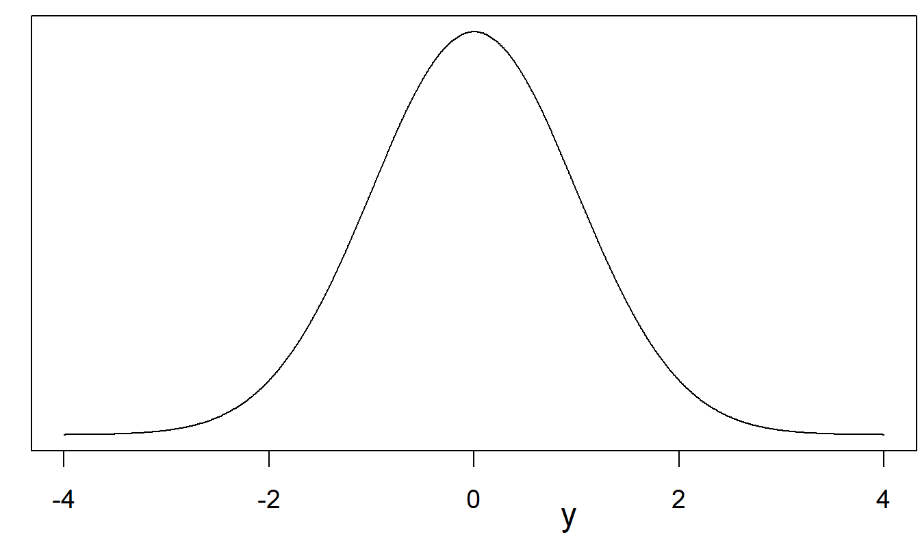
Figure 22.1: Standard normal probability density function
| x | 0.0 | 0.1 | 0.2 | 0.3 | 0.4 | 0.5 | 0.6 | 0.7 | 0.8 | 0.9 |
|---|---|---|---|---|---|---|---|---|---|---|
| 0 | 0.5000 | 0.5398 | 0.5793 | 0.6179 | 0.6554 | 0.6915 | 0.7257 | 0.7580 | 0.7881 | 0.8159 |
| 1 | 0.8413 | 0.8643 | 0.8849 | 0.9032 | 0.9192 | 0.9332 | 0.9452 | 0.9554 | 0.9641 | 0.9713 |
| 2 | 0.9772 | 0.9821 | 0.9861 | 0.9893 | 0.9918 | 0.9938 | 0.9953 | 0.9965 | 0.9974 | 0.9981 |
| 3 | 0.9987 | 0.9990 | 0.9993 | 0.9995 | 0.9997 | 0.9998 | 0.9998 | 0.9999 | 0.9999 | 1.0000 |
Notes: Probabilities can be found by looking at the appropriate row for the lead digit and column for the decimal. For example, \(\Pr ( y \le 0.1) = 0.5398\).
Chi-Square Distribution
Chi-Square Distribution. Several important distributions can be linked to the normal distribution. If \(y_1, \ldots, y_n\) are i.i.d. random variables such that each \(y_i \sim N(0,1)\), then \(\sum_{i=1}^n y_i^2\) is said to have a chi-square distribution with parameter \(n\). More generally, a random variable \(w\) with probability density function \[ \mathrm{f}(w) = \frac{2^{-k/2}}{\Gamma(k/2)} w^{k/2-1} \exp (-w/2), ~~~~~~w > 0 \] is said to have a chi-square with \(df = k\) degrees of freedom, written \(w \sim \chi_k^2\). Easy calculations show that for \(w \sim \chi_k^2\), we have \(\mathrm{E}~w = k\) and \(\mathrm{Var}~w = 2k\). In general, the degrees of freedom parameter need not be an integer, although it is for the applications of this text.
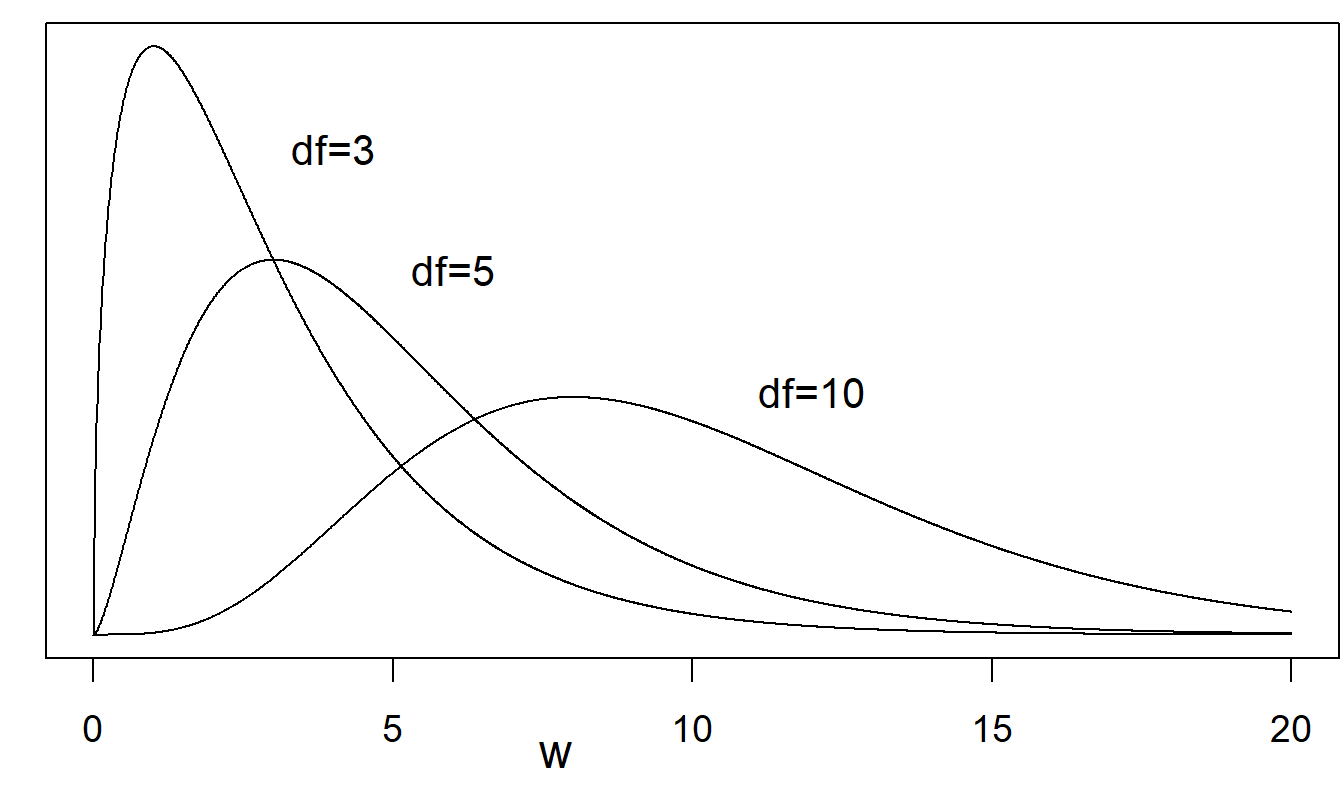
Figure 22.2: Several chi-square probability density functions. Shown are curves for \(df\) = 3, \(df\) = 5, and \(df\) = 10. Greater degrees of freedom lead to curves that are less skewed.
| df | 0.6 | 0.7 | 0.8 | 0.9 | 0.95 | 0.975 | 0.99 | 0.995 | 0.9975 | 0.999 |
|---|---|---|---|---|---|---|---|---|---|---|
| 1 | 0.71 | 1.07 | 1.64 | 2.71 | 3.84 | 5.02 | 6.63 | 7.88 | 9.14 | 10.83 |
| 2 | 1.83 | 2.41 | 3.22 | 4.61 | 5.99 | 7.38 | 9.21 | 10.60 | 11.98 | 13.82 |
| 3 | 2.95 | 3.66 | 4.64 | 6.25 | 7.81 | 9.35 | 11.34 | 12.84 | 14.32 | 16.27 |
| 4 | 4.04 | 4.88 | 5.99 | 7.78 | 9.49 | 11.14 | 13.28 | 14.86 | 16.42 | 18.47 |
| 5 | 5.13 | 6.06 | 7.29 | 9.24 | 11.07 | 12.83 | 15.09 | 16.75 | 18.39 | 20.52 |
| 10 | 10.47 | 11.78 | 13.44 | 15.99 | 18.31 | 20.48 | 23.21 | 25.19 | 27.11 | 29.59 |
| 15 | 15.73 | 17.32 | 19.31 | 22.31 | 25.00 | 27.49 | 30.58 | 32.80 | 34.95 | 37.70 |
| 20 | 20.95 | 22.77 | 25.04 | 28.41 | 31.41 | 34.17 | 37.57 | 40.00 | 42.34 | 45.31 |
| 25 | 26.14 | 28.17 | 30.68 | 34.38 | 37.65 | 40.65 | 44.31 | 46.93 | 49.44 | 52.62 |
| 30 | 31.32 | 33.53 | 36.25 | 40.26 | 43.77 | 46.98 | 50.89 | 53.67 | 56.33 | 59.70 |
| 35 | 36.47 | 38.86 | 41.78 | 46.06 | 49.80 | 53.20 | 57.34 | 60.27 | 63.08 | 66.62 |
| 40 | 41.62 | 44.16 | 47.27 | 51.81 | 55.76 | 59.34 | 63.69 | 66.77 | 69.70 | 73.40 |
| 60 | 62.13 | 65.23 | 68.97 | 74.40 | 79.08 | 83.30 | 88.38 | 91.95 | 95.34 | 99.61 |
| 120 | 123.29 | 127.62 | 132.81 | 140.23 | 146.57 | 152.21 | 158.95 | 163.65 | 168.08 | 173.62 |
t-Distribution
Suppose that \(y\) and \(w\) are independent with \(y \sim N(0,1)\) and \(w \sim \chi_k^2\). Then, the random variable \(t = y / \sqrt{w/k}\) is said to have a \(t\)-distribution with \(df = k\) degrees of freedom. The probability density function is \[ \mathrm{f}(t) = \frac{\Gamma \left( k+ \frac{1}{2} \right)}{\Gamma(k/2)} \left( k \pi \right)^{-1/2} \left( 1 + \frac{t^2}{k} \right)^{-(k+1/2)}, ~~~~~~-\infty < t < \infty \] This has mean 0, for \(k > 1\), and variance \(k/(k-2)\) for \(k > 2\).
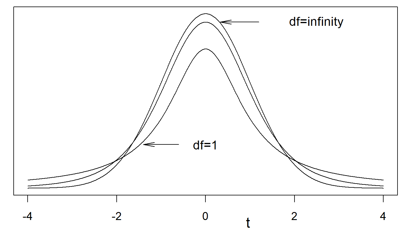
Figure 22.3: Several \(t\)-distribution probability density functions. The \(t\)-distribution with \(df = \infty\) is the standard normal distribution. Shown are curves for \(df\) = 1, \(df\) = 5 (not labeled), and \(df\) = ∞. A lower \(df\) means fatter tails.
| df | 0.6 | 0.7 | 0.8 | 0.9 | 0.95 | 0.975 | 0.99 | 0.995 | 0.9975 | 0.999 |
|---|---|---|---|---|---|---|---|---|---|---|
| 1 | 0.325 | 0.727 | 1.376 | 3.078 | 6.314 | 12.706 | 31.821 | 63.657 | 127.321 | 318.309 |
| 2 | 0.289 | 0.617 | 1.061 | 1.886 | 2.920 | 4.303 | 6.965 | 9.925 | 14.089 | 22.327 |
| 3 | 0.277 | 0.584 | 0.978 | 1.638 | 2.353 | 3.182 | 4.541 | 5.841 | 7.453 | 10.215 |
| 4 | 0.271 | 0.569 | 0.941 | 1.533 | 2.132 | 2.776 | 3.747 | 4.604 | 5.598 | 7.173 |
| 5 | 0.267 | 0.559 | 0.920 | 1.476 | 2.015 | 2.571 | 3.365 | 4.032 | 4.773 | 5.893 |
| 10 | 0.260 | 0.542 | 0.879 | 1.372 | 1.812 | 2.228 | 2.764 | 3.169 | 3.581 | 4.144 |
| 15 | 0.258 | 0.536 | 0.866 | 1.341 | 1.753 | 2.131 | 2.602 | 2.947 | 3.286 | 3.733 |
| 20 | 0.257 | 0.533 | 0.860 | 1.325 | 1.725 | 2.086 | 2.528 | 2.845 | 3.153 | 3.552 |
| 25 | 0.256 | 0.531 | 0.856 | 1.316 | 1.708 | 2.060 | 2.485 | 2.787 | 3.078 | 3.450 |
| 30 | 0.256 | 0.530 | 0.854 | 1.310 | 1.697 | 2.042 | 2.457 | 2.750 | 3.030 | 3.385 |
| 35 | 0.255 | 0.529 | 0.852 | 1.306 | 1.690 | 2.030 | 2.438 | 2.724 | 2.996 | 3.340 |
| 40 | 0.255 | 0.529 | 0.851 | 1.303 | 1.684 | 2.021 | 2.423 | 2.704 | 2.971 | 3.307 |
| 60 | 0.254 | 0.527 | 0.848 | 1.296 | 1.671 | 2.000 | 2.390 | 2.660 | 2.915 | 3.232 |
| 120 | 0.254 | 0.526 | 0.845 | 1.289 | 1.658 | 1.980 | 2.358 | 2.617 | 2.860 | 3.160 |
| ∞ | 0.253 | 0.524 | 0.842 | 1.282 | 1.645 | 1.960 | 2.326 | 2.576 | 2.807 | 3.090 |
F-Distribution
Suppose that \(w_1\) and \(w_2\) are independent with distributions \(w_1 \sim \chi_m^2\) and \(w_2 \sim \chi_n^2\). Then, the random variable \(F = (w_1/m) / (w_2/n)\) has an \(F\)-distribution with parameters \(df_1 = m\) and \(df_2 = n\), respectively. The probability density function is \[ \mathrm{f}(y) = \frac{\Gamma \left(\frac{m+n}{2} \right)}{\Gamma(m/2)\Gamma(n/2)} \left( \frac{m}{n} \right)^{m/2} \frac{y^{(m-2)/2}} {\left( 1 + \frac{m}{n}y \right)^{m+n+2}} , ~~~~~~y > 0 \] This has mean \(n/(n-2)\), for \(n > 2\), and variance \(2n^2(m+n-2)/[m(n-2)^2(n-4)]\) for \(n > 4\).
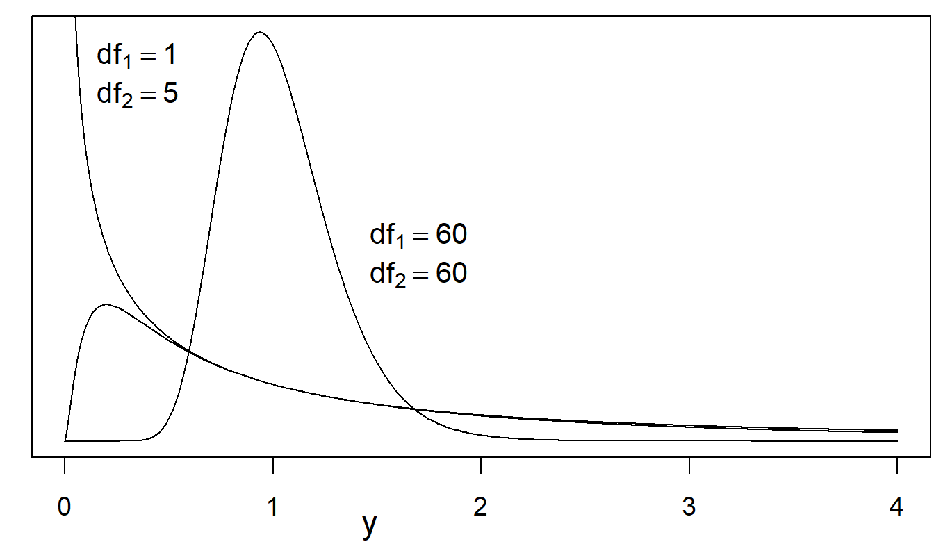
Figure 22.4: Several \(F\)-distribution probability density functions. Shown are curves for (i) \(df_1\) = 1, \(df_2\) = 5, (ii) \(df_1\) = 5, \(df_2\) = 1 (not labeled), and (iii) \(df_1\) = 60, \(df_2\) = 60. As \(df_2\) tends to \(\infty\), the \(F\)-distribution tends to a chi-square distribution.
| \(df_1\) | 1 | 3 | 5 | 10 | 20 | 30 | 40 | 60 | 120 |
|---|---|---|---|---|---|---|---|---|---|
| 1 | 161.45 | 10.13 | 6.61 | 4.96 | 4.35 | 4.17 | 4.08 | 4.00 | 3.92 |
| 2 | 199.50 | 9.55 | 5.79 | 4.10 | 3.49 | 3.32 | 3.23 | 3.15 | 3.07 |
| 3 | 215.71 | 9.28 | 5.41 | 3.71 | 3.10 | 2.92 | 2.84 | 2.76 | 2.68 |
| 4 | 224.58 | 9.12 | 5.19 | 3.48 | 2.87 | 2.69 | 2.61 | 2.53 | 2.45 |
| 5 | 230.16 | 9.01 | 5.05 | 3.33 | 2.71 | 2.53 | 2.45 | 2.37 | 2.29 |
| 10 | 241.88 | 8.79 | 4.74 | 2.98 | 2.35 | 2.16 | 2.08 | 1.99 | 1.91 |
| 15 | 245.95 | 8.70 | 4.62 | 2.85 | 2.20 | 2.01 | 1.92 | 1.84 | 1.75 |
| 20 | 248.01 | 8.66 | 4.56 | 2.77 | 2.12 | 1.93 | 1.84 | 1.75 | 1.66 |
| 25 | 249.26 | 8.63 | 4.52 | 2.73 | 2.07 | 1.88 | 1.78 | 1.69 | 1.60 |
| 30 | 250.10 | 8.62 | 4.50 | 2.70 | 2.04 | 1.84 | 1.74 | 1.65 | 1.55 |
| 35 | 250.69 | 8.60 | 4.48 | 2.68 | 2.01 | 1.81 | 1.72 | 1.62 | 1.52 |
| 40 | 251.14 | 8.59 | 4.46 | 2.66 | 1.99 | 1.79 | 1.69 | 1.59 | 1.50 |
| 60 | 252.20 | 8.57 | 4.43 | 2.62 | 1.95 | 1.74 | 1.64 | 1.53 | 1.43 |
| 120 | 253.25 | 8.55 | 4.40 | 2.58 | 1.90 | 1.68 | 1.58 | 1.47 | 1.35 |