Chapter 8 Autocorrelations and Autoregressive Models
Chapter Preview. This chapter continues our study of time series data. Chapter 7 introduced techniques for determining major patterns that provide a good first step for forecasting. Chapter 8 provides techniques for detecting subtle trends in time and models to accommodate these trends. These techniques detect and model relationships between the current and past values of a series using regression concepts.
8.1 Autocorrelations
Application: Inflation Bond Returns
To motivate the methods introduced in this chapter, we work in the context of the inflation bond return series. Beginning in January of 2003, the US Treasury Department established an inflation bond index that summarizes the returns on long-term bonds offered by the Treasury Department that are inflation-indexed. For a Treasury inflation protected security (TIPS), the principal of the bond is indexed by the (three month lagged) value of the (non-seasonally adjusted) consumer price index. The bond then pays a semi-annual coupon at a rate determined at auction when the bond is issued. The index that we examine is the unweighted average of bid yields for all TIPS with remaining terms to maturity of 10 or more years.
Monthly values of the index from January 2003 through March 2007 are considered, for a total of \(T=51\) returns. A time series plot of the data is presented in Figure 8.1. This plot suggests that the series is stationary and so it is useful to examine the distribution of the series through summary statistics that appear in Table 8.1.
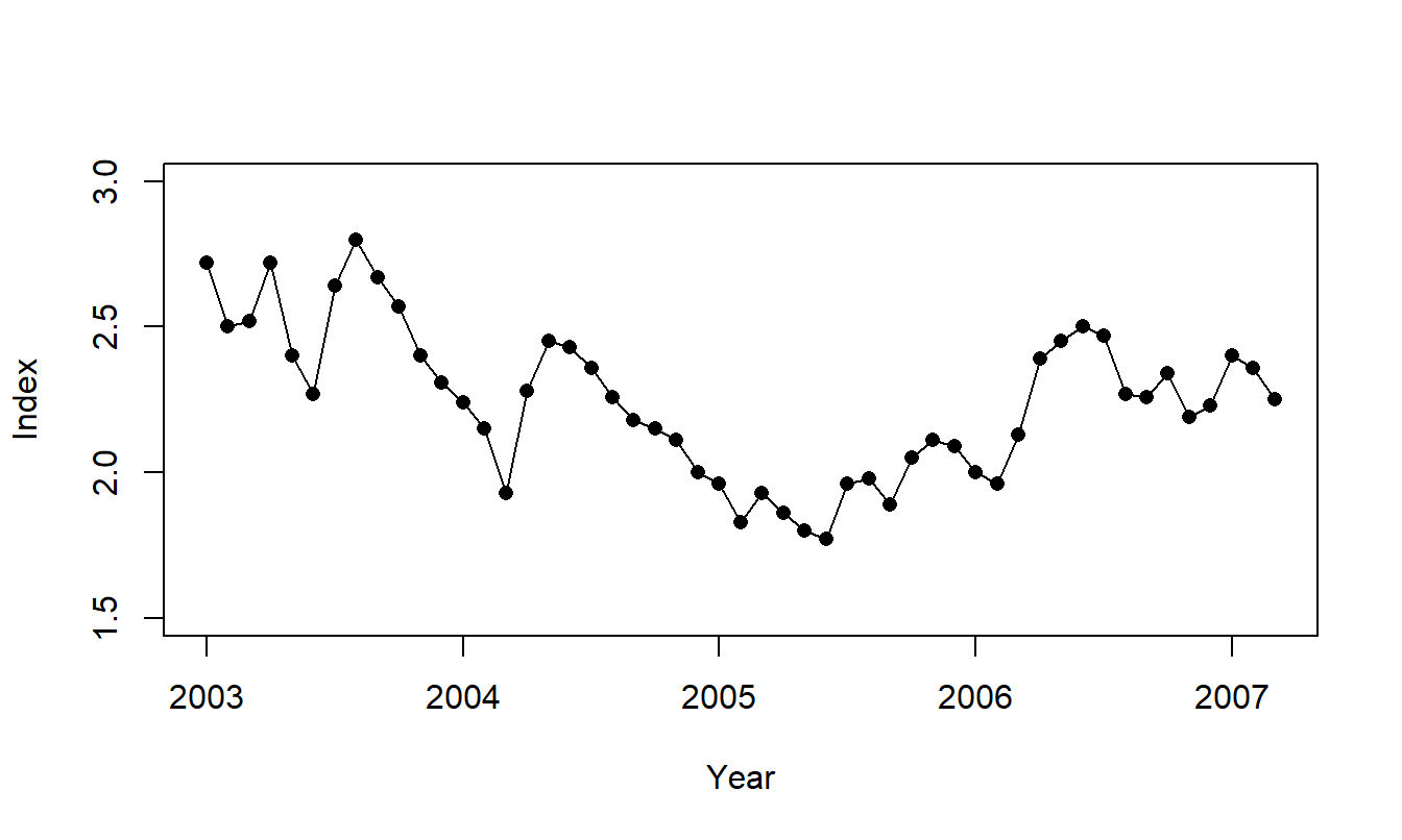
Figure 8.1: Time Series Plot of the Inflation Bond Index. Monthly values over January 2003 to March 2007, inclusive.
Table 8.1. Summary Statistics of the Inflation Bond Index
\[ \small{ \begin{array}{lccccc} \hline & & & \text{Standard} & & \\ \text{Variable} & \text{Mean} & \text{Median} & \text{Deviation} & \text{Minimum} & \text{Maximum} \\ \hline \text{INDEX} & 2.245 & 2.26 & 0.259 & 1.77 & 2.80 \\ \hline ~~~Source: \text{US Treasury} \end{array} } \]
R Code to Produce Figure 8.1 and Table 8.1
Our goal is to detect patterns in the data and provide models to represent these patterns. Although Figure 8.1 shows a stationary series with no major tendencies, a few subtle patterns are evident. Beginning in mid 2003 and then in the beginning of 2004, we see large increases followed by a series of declines in the index. Beginning in 2005, a pattern of increase with some cyclical behavior seems to be occurring. Although it is not clear what economic phenomenon these patterns represent, they are not what we would expect to see with a white noise process. For a white noise process, a series may increase or decrease randomly from one period to the next, producing a non-smooth, “jagged” series over time.
To help understand these patterns, Figure 8.2 presents a scatter plot of the series (\(y_t\)) versus its lagged value (\(y_{t-1}\)). Because this is a crucial step to understanding this chapter, Table 8.2 presents a small subset of the data so that you can see exactly what each point on the scatter plot represents. Figure 8.2 shows a strong relationship between \(y_t\) and \(y_{t-1}\); we will model this relationship in the next section.
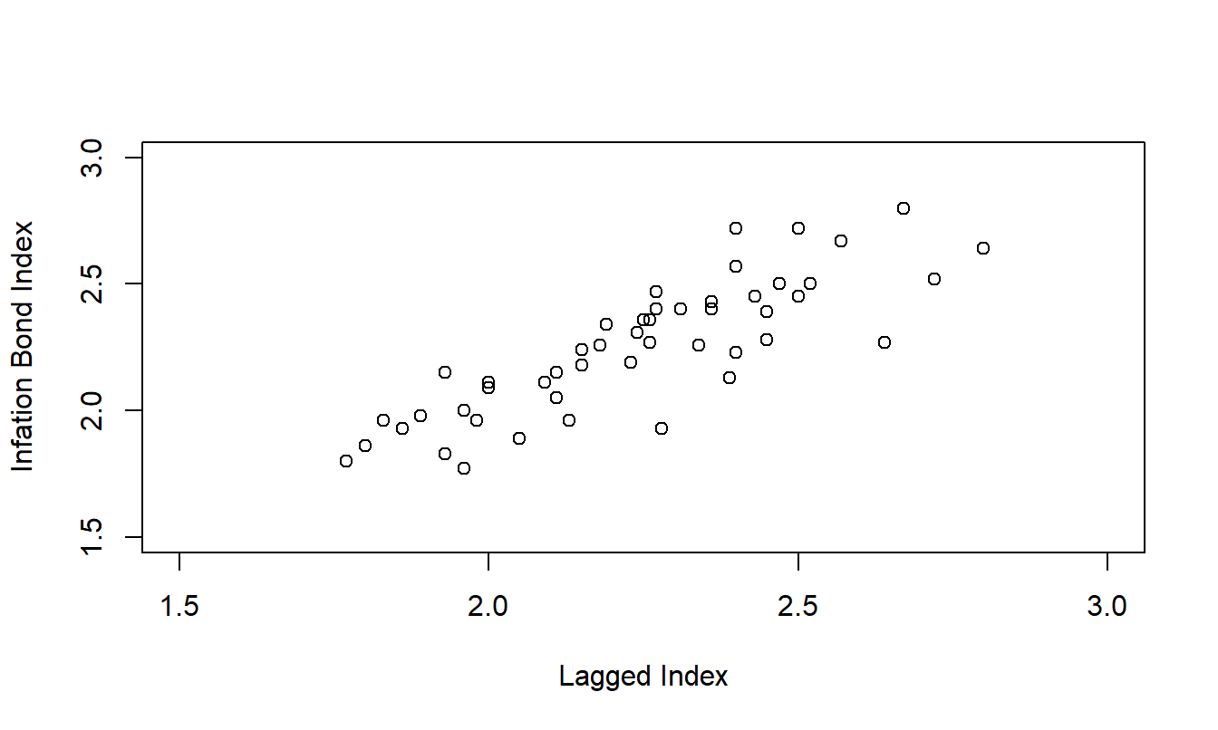
Figure 8.2: Inflation Bond versus Lagged Value. This scatter plot reveals a linear relationship between the index and its lagged value
Table 8.2. Index and Lagged Index for the First Five of \(T=51\) Values
\[ \small{ \begin{array}{l|crrrr} \hline t & 1~~ & 2~~ & 3~~ & 4~~ & 5~~ \\ \hline \text{Index }(y_t) & 2.72 & 2.50 & 2.52 & 2.72 & 2.40 \\ \text{Lagged Index } (y_{t-1}) & * & 2.72 & 2.50 & 2.52 & 2.72 \\ \hline \end{array} } \]
R Code to Produce Figure 8.2
Autocorrelations
Scatter plots are useful because they graphically display nonlinear, as well as linear, relationships between two variables. As we established in Chapter 2, correlations can be used to measure the linear relation between two variables. Recall that when dealing with cross-sectional data, we summarized relations between {\(y_t\)} and {\(x_t\)} using the correlation statistic \[ r = \frac{1}{(T-1)s_{x}s_y} \sum_{t=1}^{T} \left( x_t - \overline{x}\right) \left( y_t-\overline{y} \right) . \] We now mimic this statistic using the series {\(y_{t-1}\)} in place of {\(x_t\)}. With this replacement, use \(\overline{y}\) in place of \(\overline{x}\) and, for the denominator, use \(s_y\) in place of \(s_x\). With this last substitution, we have \((T-1) s_y^2 = \sum_{t=1}^{T}(y_t-\overline{y} )^2\). Our resulting correlation statistic is
\[ r_1 = \frac{\sum_{t=2}^{T} \left( y_{t-1}-\overline{y}\right) \left( y_t- \overline{y}\right) }{\sum_{t=1}^{T} (y_t-\overline{y})^2}. \] This statistic is referred to as an autocorrelation, that is, a correlation of the series upon itself. This statistic summarizes the linear relationship between {\(y_t\)} and {\(y_{t-1}\)}, that is, observations that are one time unit apart. It will also be useful to summarize the linear relationship between observations that are \(k\) time units apart, {\(y_t\)} and {\(y_{t-k}\)}, as follows.
Definition. The lag k autocorrelation statistic is
\[ r_k = \frac{\sum_{t=k+1}^{T}\left( y_{t-k}-\overline{y}\right) \left( y_t- \overline{y}\right) }{\sum_{t=1}^{T}(y_t-\overline{y})^2}, ~~~~k=1,2, \ldots \]
Properties of autocorrelations are similar to correlations. Just as with the usual correlation statistic \(r\), the denominator, \(\sum_{t=1}^{T}(y_t - \overline{y})^2\), is always nonnegative and hence does not change the sign of the numerator. We use this rescaling device so that \(r_k\) always lies within the interval [-1, 1]. Thus, when we interpret \(r_k\), a value near -1, 0 and 1, means, respectively, a strong negative, near null or strong positive relationship between \(y_t\) and \(y_{t-k}\). If there is a positive relationship between \(y_t\) and \(y_{t-1}\), then \(r_1 > 0\) and the process is said to be positively autocorrelated. For example, in Table 8.3 are the first five autocorrelations of the inflation bond series. These autocorrelations indicate that there is a positive relationship between adjacent observations.
Table 8.3. Autocorrelations for the Inflation Bond Series
\[ \small{ \begin{array}{l|ccccc} \hline \text{Lag } k & 1 & 2 & 3 & 4 & 5 \\ \hline \text{Autocorrelation } r_k & 0.814 & 0.632 & 0.561 & 0.447 & 0.367 \\ \hline \end{array} } \]
R Code to Produce Table 8.3
Video: Section Summary
8.2 Autoregressive Models of Order One
Model Definition and Properties
In Figure 8.2 we noted the strong relationship between the immediate past and current values of the inflation bond index. This suggests using \(y_{t-1}\) to explain \(y_t\) in a regression model. Using previous values of a series to predict current values of a series is termed, not surprisingly, an autoregression. When only the immediate past is used as a predictor, we use the following model.
Definition. The autoregressive model of order one, denoted by \(AR(1)\), is written as \[\begin{equation} y_t = \beta_0 + \beta_1 y_{t-1} + \varepsilon_t, ~~~ t=2,\ldots,T, \tag{8.1} \end{equation}\] where {\(\varepsilon_t\)} is a white noise process such that \(\mathrm{Cov}(\varepsilon_{t+k}, y_t)=0\) for \(k>0\) and \(\beta_0\) and \(\beta_1\) are unknown parameters.
In the \(AR\)(1) model, the parameter \(\beta_0\) may be any fixed constant. However, the parameter \(\beta_1\) is restricted to be between -1 and 1. By making this restriction, it can be established that the \(AR\)(1) series {\(y_t\)} is stationary. Note that if \(\beta_1 = 1\), then the model is a random walk and hence is nonstationary. This is because, if \(\beta_1 = 1\), then equation (8.1) may be rewritten as \[ y_t - y_{t-1} = \beta_0 + \varepsilon_t. \] If the difference of a series forms a white noise process, then the series itself must be a random walk.
The equation (8.1) is useful in the discussion of model properties. We can view an \(AR\)(1) model as a generalization of both a white noise process and a random walk model. If \(\beta_1=0\), then equation (8.1) reduces to a white noise process. If \(\beta_1 = 1,\) then equation (8.1) is a random walk.
A stationary process where there is a linear relationship between \(y_{t-2}\) and \(y_t\) is said to be autoregressive of order 2, and similarly for higher order processes. Discussion of higher order processes is in Section 8.5.
Model Selection
When examining the data, how does one recognize that an autoregressive model may be a suitable candidate model? First, an autoregressive model is stationary and thus a control chart is a good device to examine graphically the data to search for stability. Second, adjacent realizations of an \(AR\)(1) model should be related; this can be detected visually by a scatter plot of current versus immediate past values of the series. Third, we can recognize an \(AR\)(1) model through its autocorrelation structure, as follows.
A useful property of the \(AR\)(1) model is that the correlation between points \(k\) time units apart turns out to be \(\beta_1^{k}\). Stated another way, \[\begin{equation} \rho_k = \mathrm{Corr}(y_t,y_{t-k}) = \frac{\mathrm{Cov}(y_t,y_{t-k})}{\sqrt{\mathrm{Var}(y_t)\mathrm{Var}(y_{t-k})}} = \frac{\mathrm{Cov}(y_t,y_{t-k})}{\sigma_y^2} = \beta_1^k. \tag{8.2} \end{equation}\]
The first two equalities are definitions and the third is due to the stationarity. The reader is asked to check the fourth equality in the exercises. Hence, the absolute values of the autocorrelations of an \(AR\)(1) process become smaller as the lag time \(k\) increases. In fact, they decrease at a geometric rate. We remark that for a white noise process, we have \(\beta_1 = 0\), and thus \(\rho_k\) should be equal to zero for all lags \(k\).
As an aid in model identification, we use the idea of matching the observed autocorrelations \(r_k\) to quantities that we expect from the theory, \(\rho_k\). For white noise, the sample autocorrelation coefficient should be approximately zero for each lag \(k\). Even though \(r_k\) is algebraically bounded by -1 and 1, the question arises, how large does \(r_k\) need to be, in absolute value, to be considered significantly different from zero? The answer to this type of question is given in terms of the statistic’s standard error. Under the hypothesis of no autocorrelation, a good approximation to the standard error of the lag \(k\) autocorrelation statistic is \[ se(r_k) = \frac{1}{\sqrt{T}}. \] Our rule of thumb is that if \(r_k\) exceeds \(2 \times se(r_k)\) in absolute value, it may be considered to be significantly non-zero. This rule is based on a 5% level of significance.
Example: Inflation Index Bonds - Continued. Is a white noise process model a good candidate to represent this series? The autocorrelations are given in Table 8.2. For a white noise process model, we expect each autocorrelation \(r_k\) to be close to zero but note that, for example, \(r_1=0.814\). Because there are \(T=51\) returns available, the approximate standard error of each autocorrelation is \[ se(r_k) = \frac{1}{\sqrt{51}} = 0.140. \] Thus, \(r_1\) is 0.814 / 0.140 = 5.81 standard errors above zero. Using the normal distribution as a reference base, this difference is significant, implying that a white noise process is not a suitable candidate model.
Is the autoregressive model of order one a suitable choice? Well, because \(\rho_k\) = \(\beta_1^{k}\), a good estimate of \(\beta_1\)=\(\rho_1\) is \(r_1=0.814\). If this is the case, then under the \(AR\)(1) model, another estimate of \(\rho_k\) is \((0.814)^{k}\). Thus, we have two estimates of \(\rho_k\); (i) \(r_k\), an empirical estimate that does not depend on a parametric model and (ii) \((r_1)^{k}\), that depends on the \(AR\)(1) model. To illustrate, see Table 8.4.
Table 8.4. Comparison of Empirical Autocorrelations to Estimated under the \(AR\)(1) model
\[ \small{ \begin{array}{l|ccccc} \hline \text{Lag } k & 1 & 2 & 3 & 4 & 5 \\ \hline \text{Estimated } \rho_k \text{ under the } AR(1) \text{ model} & 0.814 & (0.814)^2 & (0.814)^{3} & (0.814)^{4} & (0.814)^{5} \\ & & =.66 & =.54 & =.44 & =.36 \\ \text{Autocorrelation } r_k & 0.814 & 0.632 & 0.561 & 0.447 & 0.367 \\ \hline \end{array} } \]
Given that the approximate standard error is \(se(r_k) = 0.14\), there seems to be a good match between the two sets of autocorrelations. Because of this match, in Section 8.3 we will discuss how to fit the \(AR\)(1) model to this set of data.
Meandering Process
Many processes display the pattern of adjacent points being related to one another. Thinking of a process evolving as a river, Roberts (1991) picturesquely describes such processes as meandering. To supplement this intuitive notion, we say that a process is meandering if the lag one autocorrelation of the series is positive. For example, from the plots in Figures 8.1 and 8.2, it seems clear that the Inflation Bond Index is a good example of a meandering series. Indeed, an \(AR\)(1) model with a positive slope coefficient is a meandering process.
What about the case when the slope coefficient approaches one, resulting in a random walk? Consider the Hong Kong Exchange Rates example given in Chapter 7. Although introduced as a quadratic trend in time model, an exercise shows that the series can more appropriately be modeled as a random walk. It seems clear that any point in the process is highly related to each adjacent point in the process. To emphasize this point, Figure 8.3 shows a strong linear relationship between the current and immediate past value of exchange rates. Because of the strong linear relationship in Figure 8.3, we will use the terminology “meandering process” for a data set that may be modeled using a random walk.
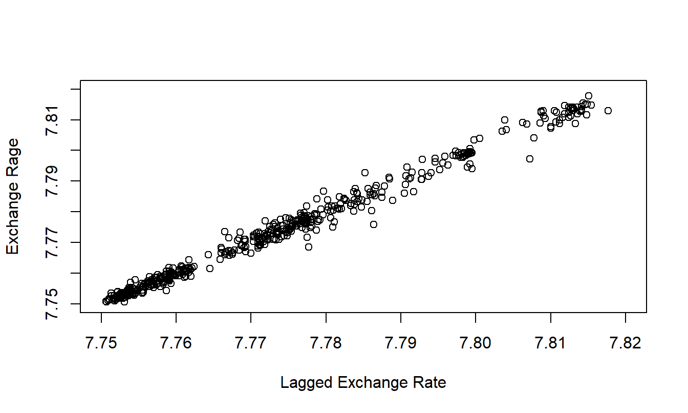
Figure 8.3: Hong Kong Daily Exchange Rates versus Lagged Values.
R Code to Produce Figure 8.3
Video: Section Summary
8.3 Estimation and Diagnostic Checking
Having identified a tentative model, the task now at hand is to estimate values of \(\beta_0\) and \(\beta_1\). In this section, we use the method of conditional least squares to determine the estimates, denoted as \(b_0\) and \(b_1\), respectively. This approach is based on the least squares method that was introduced in Section 2.1. Specifically, we now use the least squares to find estimates that best fit an observation conditional on the previous observation.
Formulas for the conditional least squares estimates are determined from the usual least squares procedures, using the lagged value of \(y\) for the explanatory variable. It is easy to see that conditional least squares estimates are closely approximated by \[ b_1 \approx r_1 \ \ \ \ \ \ \text{and} \ \ \ \ \ \ b_0 \approx \overline{y}(1-r_1). \] Differences between these approximations and the conditional least squares estimates arise because we have no explanatory variable for \(y_1\), the first observation. These differences are typically small in most series and diminish as the series length increases.
Residuals of an \(AR\)(1) model are defined as \[ e_t = y_t - \left( b_0 + b_1 y_{t-1} \right). \] As we have seen, patterns in the residuals may reveal ways to improve the model specification. One can use a control chart of the residuals to assess the stationarity and compute the autocorrelation function of residuals to verify the lack of milder patterns through time.
The residuals also play an important role in estimating standard errors associated with model parameter estimates. From equation (8.1), we see that the unobserved errors are driving the updating of the new observations. Thus, it makes sense to focus on the variance of the errors and, as in cross-sectional data, we define \(\sigma^2=\sigma_{\varepsilon }^2=\) \(\mathrm{Var}~\varepsilon_t.\)
In cross-sectional regression, because the predictor variables were non-stochastic, the variance of the response (\(\sigma_y^2\)) equals the variance of the errors (\(\sigma^2\)). This is not generally true in time series models that use stochastic predictors. For the \(AR\)(1) model, taking variances of both sides of equation (8.1) establishes \[ \sigma_y^2 (1-\beta_1^2) = \sigma^2 , \] so that \(\sigma_y^2 > \sigma^2\).
To estimate \(\sigma^2\), we define \[\begin{equation} s^2 = \frac{1}{T-3}\sum_{t=2}^{T} \left( e_t - \overline{e}\right)^2. \tag{8.3} \end{equation}\] In equation (8.3) the first residual, \(e_1\), is not available because \(y_{t-1}\) is not available when \(t=1\) and so the number of residuals is \(T-1\). Without the first residual, the average of the residuals is no longer automatically zero and thus is included in the sum of squares. Further, the denominator in the right hand side of equation (8.3) is still the number of observations minus the number of parameters, keeping in mind the conditions that the “number of observations” is \(T-1\) and the “number of parameters” is two. As in the cross-sectional regression context, we refer to \(s^2\) as the mean square error (MSE).
Example: Inflation Index Bonds - Continued. The inflation index was fit using an \(AR\)(1) model. The estimated equation turns out to be \[ \begin{array}{llllrl} \widehat{INDEX}_t & = & 0.40849 & + & 0.81384 & INDEX_{t-1} \\ {\small std~errors} & & {\small (0.16916)} & & {\small (0.07486)} & \end{array} \] with \(s = 0.14\). This is smaller than the standard deviation of the original series (0.259 from Table 8.1), indicating a better fit to the data than a white noise model. The standard errors, given in parentheses, were computed using the method of conditional least squares. For example, the \(t\)-ratio for \(\beta_1\) is \(0.8727/0.0736=14.9\), indicating that the immediate past response is an important predictor of the current response.
Residuals were computed as \(e_t = INDEX_t - (0.2923+0.8727INDEX_{t-1})\). The control chart of the residuals in Figure 8.4 reveals no apparent patterns. Several autocorrelations of residuals are presented in Table 8.5. With \(T=51\) observations, the approximate standard error is \(se(r_k) = 1/ \sqrt{51} = 0.14\). The second lag autocorrelation is approximately -2.3 standard errors from zero and the others are smaller, in absolute value. These values are lower than those in Table 8.3, indicating that we have removed some of the temporal patterns with the \(AR\)(1) specification. The statistically significant autocorrelation at lag 2 indicates that there is still some potential for model improvement.
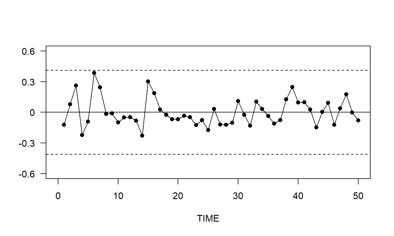
Figure 8.4: Control Chart of Residuals from an \(AR\)(1) Fit of the Inflation Index Series. The dashed lines mark the upper and lower control limits which are the mean plus and minus three standard deviations.
Table 8.5. Residual Autocorrelations from the \(AR\)(1) model
\[ \small{ \begin{array}{l|ccccc} \hline \text{Lag }k & 1 & 2 & 3 & 4 & 5 \\ \hline \text{Residual Autocorrelation }r_k & 0.157 &-0.289 & 0.059 & 0.073& -0.124 \\ \hline \end{array} } \]
R Code to Produce Figure 8.4 and Table 8.5
Video: Section Summary
8.4 Smoothing and Prediction
Having identified, fit, and checked the identification of the model, we now proceed to basic inference. Recall that by inference we mean the process of using the data set to make statements about the nature of the world. To make statements about the series, analysts often examine the values fitted under the model, called the smoothed series. The smoothed series is the estimated expected value of the series given the past. For the \(AR\)(1) model, the smoothed series is \[ \widehat{y}_t=b_0+b_1y_{t-1}. \]
In Figure 8.5, an open circle represents the actual Inflation Bond Index and an opaque circle represents the corresponding smoothed series. Because the smoothed series is the actual series with the estimated noise component removed, the smoothed series is sometimes interpreted to represent the “real” value of the series.
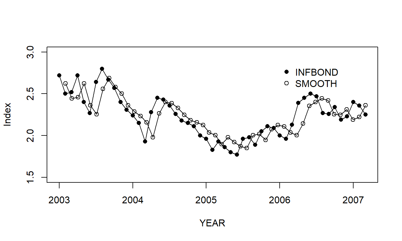
Figure 8.5: Inflation Bond Index with a Smoothed Series Superimposed. The index is given by the open plotting symbols, the smoothed series is represented by the opaque symbols.
R Code to Produce Figure 8.5
Typically, the most important application of time series modeling is the forecasting of future values of the series. From equation (8.1), the immediate future value of the series is \(y_{T+1} = \beta_0 + \beta_1 y_T + \varepsilon_{T+1}\). Because the series {\(\varepsilon_t\)} is random, a natural forecast of \(\varepsilon_{T+1}\) is its mean, zero. Thus, if the estimates \(b_0\) and \(b_1\) are close to the true parameters \(\beta_0\) and \(\beta_1\), then a desirable estimate of the series at time \(T+1\) is \(\widehat{y}_{T+1} = b_0 + b_1 y_T\). Similarly, one can recursively compute an estimate for the series \(k\) time points in the future, \(y_{T+k}\).
Definition. The \(k\)-step ahead forecast of \(y_{T+k}\) for an \(AR\) (1) model is recursively determined by \[\begin{equation} \widehat{y}_{T+k} = b_0 + b_1 \widehat{y}_{T+k-1}. \tag{8.4} \end{equation}\] This is sometimes known as the chain rule of forecasting.
To get an idea of the error in using \(\widehat{y}_{T+1}\) to predict \(y_{T+1}\), assume for the moment that the error in using \(b_0\) and \(b_1\) to estimate \(\beta_0\) and \(\beta_1\) is negligible. With this assumption, the forecast error is \[ y_{T+1}-\widehat{y}_{T+1} = \beta_0 + \beta_1 y_t + \varepsilon_{T+1} - \left( b_0 + b_1 y_t\right) \approx \varepsilon_{T+1}. \] Thus, the variance of this forecast error is approximately \(\sigma^2\). Similarly, it can be shown that the approximate variance of the forecast error \(y_{T+k}-\widehat{y}_{T+k}\) is \(\sigma^2(1 + \beta_1^2 \ldots + \beta_1^{2(k-1)})\). From this variance calculation and the approximate normality, we have the following prediction interval.
Definition. The \(k\)-step ahead forecast interval of \(y_{T+k}\) for an \(AR\)(1) model is \[ \widehat{y}_{T+k} \pm (t-value)~s \sqrt{1 + b_1^2+ \ldots + b_1^{2(k-1)}}. \] Here, the \(t\)-value is a percentile from the \(t\)-curve using \(df=T-3\) degrees of freedom. The percentile is 1 - (prediction level)/2.
For example, for 95% prediction intervals, we would have \(t\)-value \(\approx\) 2. Thus, one- and two-step 95% prediction intervals are: \[ \begin{array}{lc} \text{one-step:} & \widehat{y}_{T+1}\pm \ 2s \\ \text{two-step:} & \widehat{y}_{T+2}\pm \ 2s(1+b_1^2)^{1/2}. \end{array} \]
Figure 8.6 illustrates forecasts of the inflation bond index. The forecast intervals widen as the number of steps into the future increases; this reflects our increasing uncertainty as we forecast further into the future.
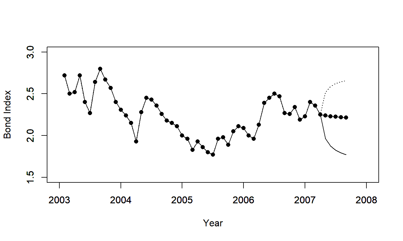
Figure 8.6: Forecast Intervals for the Inflation Bond Series.
R Code to Produce Figure 8.6
Video: Section Summary
8.5 Box-Jenkins Modeling and Forecasting
Sections 8.1 through 8.4 introduced the \(AR(1)\) model, including model properties, identification methods and forecasting. We now introduce a broader class of models known as autoregressive integrated moving average (ARIMA) models, due to George Box and Gwilym Jenkins, see Box, Jenkins and Reinsel (1994).
8.5.1 Models
\(AR(p)\) Models
The autoregressive model of order one allows us to relate the current behavior of an observation directly to its immediate past value. Moreover, in some applications, there are also important effects of observations that are more distant in the past than simply the immediate preceding observation. To quantify this, we have already introduced the lag \(k\) autocorrelation \(\rho_k\) that captures the linear relationship between \(y_t\) and \(y_{t-k}\). To incorporate this feature into a forecasting framework, we have the autoregressive model of order p, denoted by \(AR(p).\) The model equation is \[\begin{equation} y_t = \beta_0 + \beta_1 y_{t-1} + \ldots + \beta_p y_{t-p} + \varepsilon_t, ~~~~ t=p+1,\ldots ,T, \tag{8.5} \end{equation}\] where {\(\varepsilon_t\)} is a white noise process such that \(\mathrm{Cov}(\varepsilon_{t+k}, y_t)=0\) for \(k>0\) and \(\beta_0\), \(\beta_1,\ldots,\beta_p\) are unknown parameters.
As a convention, when data analysts specify an \(AR\)(\(p\)) model, they include not only \(y_{t-p}\) as a predictor variable, but also the intervening lags, \(y_{t-1}, \ldots, y_{t-p+1}\). The exceptions to this convention are the seasonal autoregressive models, that will be introduced in Section 9.4. Also by convention, the \(AR(p)\) is a model of a stationary, stochastic process. Thus, certain restrictions on the parameters \(\beta_1, \ldots, \beta_p\) are necessary to ensure (weak) stationarity. These restrictions are developed in the following subsection.
Backshift Notation
The backshift, or backwards-shift, operator \(\mathrm{B}\) is defined by \(\mathrm{B}y_t\) = \(y_{t-1}\). The notation \(\mathrm{B}^{k}\) means apply the operator \(k\) times, that is, \[ \mathrm{B}^{k}~y_t = \mathrm{BB \cdots B~} y_t = \mathrm{B} ^{k-1}~y_{t-1} = \cdots = y_{t-k}. \] This operator is linear in the sense that \(\mathrm{B} (a_1 y_t + a_2 y_{t-1}) = a_1 y_{t-1} + a_2 y_{t-2}\), where \(a_1\) and \(a_2\) are constants. Thus, we can express the \(AR(p)\) model as \[\begin{eqnarray*} \beta_0 + \varepsilon_t &=& y_t - \left( \beta_1 y_{t-1} + \ldots + \beta_p y_{t-p}\right) \\ &=& \left(1-\beta_1 \mathrm{B} - \ldots - \beta_p \mathrm{B}^{p}\right) y_t = \Phi \left( \mathrm{B}\right) y_t. \end{eqnarray*}\] If \(x\) is a scalar, then \(\Phi \left( x\right) = 1 - \beta_1 x - \ldots - \beta_p x^p\) is a \(p\)th order polynomial in \(x\). Thus, there exist \(p\) roots of the equation \(\Phi \left( x\right) =0\). These roots, say, \(g_1,..,g_p\) , may or may not be complex numbers. It can be shown, see Box, Jenkins and Reinsel (1994), that for stationarity, all roots lie strictly outside the unit circle. To illustrate, for \(p=1\), we have \(\Phi \left( x\right) = 1 - \beta_1 x\). The root of this equation is \(g_1 = \beta_1^{-1}\). Thus, we require \(|g_1|>1\), or \(|\beta_1|<1\), for stationarity.
\(MA(q)\) Models
One interpretation of the model \(y_t=\beta_0+\varepsilon_t\) is that the disturbance \(\varepsilon_t\) perturbs the measure of the true, expected value of \(y_t.\) Similarly, we can consider the model \(y_t=\beta_0 + \varepsilon _t-\theta_1\varepsilon_{t-1}\), where \(\theta_1 \varepsilon_{t-1}\) is the perturbation from the previous time period. Extending this line of thought, we introduce the moving average model of order q, denoted by \(MA(q)\). The model equation is \[\begin{equation} y_t = \beta_0 + \varepsilon_t - \theta_1 \varepsilon_{t-1} - \ldots - \theta_q \varepsilon_{t-q}, \tag{8.6} \end{equation}\] where the process {\(\varepsilon_t\)} is a white noise process such that \(\mathrm{Cov}(\varepsilon_{t+k}, y_t)=0\) for \(k>0\) and \(\beta_0\), \(\theta_1, \ldots, \theta_q\) are unknown parameters.
With equation (8.6) it is easy to see that \(\mathrm{Cov} (y_{t+k},y_t)=0\) for \(k>q\). Thus, \(\rho_k =0\) for \(k>q\). Unlike the \(AR(p)\) model, the \(MA(q)\) process is stationary for any finite values of the parameters \(\beta_0\), \(\theta_1, \ldots, \theta_q\). It is convenient to write the \(MA(q)\) using backshift notation, as follows: \[ y_t - \beta_0 = \left( 1-\theta_1\mathrm{B} - \ldots - \theta_q \mathrm{B}^q\right) \varepsilon_t = \Theta \left( \mathrm{B}\right) \varepsilon_t. \] As with \(\Phi \left( x\right)\), if \(x\) is a scalar, then \(\Theta \left( x\right) = 1 - \theta_1 x - \ldots - \theta_q x^q\) is a \(q\)th order polynomial in \(x\). It is unfortunate that the phrase “moving average” is used for the model defined by equation (8.6) and the estimate defined in Section 9.2. We will attempt to clarify the usage as it arises.
\(ARMA\) and \(ARIMA\) Models
Combining the \(AR(p)\) and the \(MA(q)\) models yields the autoregressive moving average model of order \(p\) and \(q\), or \(ARMA(p,q)\), \[\begin{equation} y_t - \beta_1 y_{t-1} - \ldots - \beta_p y_{t-p} = \beta_0 + \varepsilon _t - \theta_1 \varepsilon_{t-1} - \ldots - \theta_q \varepsilon_{t-q}, \tag{8.7} \end{equation}\] which can be represented as \[\begin{equation} \Phi \left( \mathrm{B}\right) y_t = \beta_0 + \Theta \left( \mathrm{B} \right) \varepsilon_t. \tag{8.8} \end{equation}\]
In many applications, the data requires differencing to exhibit stationarity. We assume that the data are differenced \(d\) times to yield \[\begin{equation} w_t = \left( 1-\mathrm{B}\right)^d y_t = \left( 1-\mathrm{B}\right) ^{d-1}\left( y_t-y_{t-1}\right) = \left( 1-\mathrm{B}\right) ^{d-2}\left( y_t-y_{t-1}-\left( y_{t-1}-y_{t-2}\right) \right) = \ldots \tag{8.9} \end{equation}\] In practice, \(d\) is typically zero, one or two. With this, the autoregressive integrated moving average model of order \((p,d,q)\), denoted by \(ARIMA(p,d,q)\), is \[\begin{equation} \Phi \left( \mathrm{B}\right) w_t = \beta_0+\Theta \left( \mathrm{B} \right) \varepsilon_t. \tag{8.10} \end{equation}\] Often, \(\beta_0\) is zero for \(d>0\).
Several procedures are available for estimating model parameters including maximum likelihood estimation, and conditional and unconditional least squares estimation. In most cases, these procedures require iterative fitting procedures. See Abraham and Ledolter (1983) for further information.
Example: Forecasting Mortality Rates. To quantify values in life insurance and annuities, actuaries need forecasts of age-specific mortality rates. Since its publication, the method proposed by Lee and Carter (1992) has proved to be a popular method to forecast mortality. For example, Li and Chan (2007) used these methods to produce forecasts of 1921-2000 Canadian population rates and 1900-2000 U.S. rates. They showed how to modify the basic methodology to incorporate atypical events including wars and pandemic events such as influenza and pneumonia.
The Lee-Carter method is usually based on central death rates at age \(x\) at time \(t\), denoted by \(m_{x,t}\). The model equation is \[\begin{equation} m_{x,t} = \alpha_x + \beta_x \kappa_t + \varepsilon_{x,t} . \tag{8.11} \end{equation}\] Here, the intercept (\(\alpha_x\)) and slope (\(\beta_x\)) depend only on age \(x\), not on time \(t\). The parameter \(\kappa_t\) captures the important time effects (except for those in the disturbance term \(\varepsilon_{x,t}\)).
At first glance, the Lee-Carter model appears to be a linear regression with one explanatory variable. However, the term \(\kappa_t\) is not observed and so different techniques are required for model estimation. Different algorithms are available, including the singular value decomposition proposed by Lee and Carter, the principal components approach and a Poisson regression model; see Li and Chan (2007) for references.
The time-varying term \(\kappa_t\) is typically represented using an \(ARIMA\) model. Li and Chan found that a random walk (with adjustments for unusual events) was a suitable model for Canadian and U.S. rates (with different coefficients), reinforcing the findings of Lee and Carter.
8.5.2 Forecasting
Optimal Point Forecasts
Similar to forecasts that were introduced in Section 8.4, it is common to provide forecasts that are estimates of conditional expectations of the predictive distribution. Specifically, assume we have available a realization of {\(y_1, y_2, \ldots, y_T\)} and would like to forecast \(y_{T+l}\), the value of the series “\(l\)” lead time units in the future. If the parameters of the process were known, then we would use \(\mathrm{E}(y_{T+l}|y_T,y_{T-1},y_{T-2},\ldots)\), that is, the conditional expectation of \(y_{T+l}\) given the value of the series up to and including time \(T\). We use the notation \(\mathrm{E}_T\) for this conditional expectation.
To illustrate, taking \(t=T+l\) and applying \(\mathrm{E}_T\) to both sides of equation (8.7) yields \[\begin{equation} y_T(l) - \beta_1 y_T(l-1) - \ldots - \beta_p y_T(l-p) = \beta_0 + \mathrm{E}_T\left( \varepsilon_{T+l} - \theta_1 \varepsilon_{T+l-1} - \ldots - \theta _q \varepsilon_{T+l-q}\right) , \tag{8.12} \end{equation}\] using the notation \(y_T(k) = \mathrm{E}_T\left( y_{T+k}\right)\). For \(k \leq 0\), \(\mathrm{E}_T\left( y_{T+k}\right) =y_{T+k}\), as the value of \(y_{T+k}\) is known at time \(T\). Further, \(\mathrm{E}_T\left( \varepsilon_{T+k}\right) =0\) for \(k>0\) as disturbance terms in the future are assumed to be uncorrelated with current and past values of the series. Thus, equation (8.12) provides the basis of the chain rule of forecasting, where we recursively provide forecasts at lead time \(l\) based on prior forecasts and realizations of the series. To implement equation (8.12), we substitute estimates for parameters and residuals for disturbance terms.
Special Case - MA(1) Model. We have already seen the forecasting chain rule for the \(AR(1)\) model in Section 8.4. For the \(MA(1)\) model, note that for \(l\geq 2\), we have \(y_T(l)=\mathrm{E}_T\left( y_{T+l}\right)\) \(=\mathrm{E}_T\left( \beta_0+\varepsilon_{T+l}-\theta_1\varepsilon_{T+l-1}\right) =\beta_0\), because \(\varepsilon_{T+l}\) and \(\varepsilon _{T+l-1}\) are in the future at time \(T\). For \(l=1\), we have \(y_T(1)= \mathrm{E}_T\left( \beta_0+\varepsilon_{T+1}-\theta _1\varepsilon_T\right)\) \(=\beta_0-\theta_1\mathrm{E}_T\left( \varepsilon_T\right)\). Typically, one would estimate the term \(\mathrm{E}_T\left( \varepsilon_T\right)\) using the residual at time \(T\).
\(\psi\)-Coefficient Representation
Any \(ARIMA(p,d,q)\) model can be expressed as \[ y_t=\beta_0^{\ast }+\varepsilon_t+\psi_1 \varepsilon_{t-1}+\psi _2\varepsilon_{t-2}+\ldots=\beta_0^{\ast }+\sum_{k=0}^{\infty }\psi _{k}\varepsilon_{t-k}, \] called the \(\psi\)-coefficient representation. That is, the current value of a process can be expressed as a constant plus a linear combination of the current and previous disturbances. Values of {\(\psi_{k}\)} depend on the linear parameters of the \(ARIMA\) process and can be determined via straightforward recursive substitution. To illustrate, for the \(AR(1)\) model, we have \[\begin{eqnarray*} y_t &=&\beta_0+\varepsilon_t+\beta_1y_{t-1}=\beta_0+\varepsilon _t+\beta_1\left( \beta_0+\varepsilon _{t-1}+\beta_1y_{t-2}\right) =\ldots \\ &=&\frac{\beta_0}{1-\beta_1}+\varepsilon_t+\beta_1\varepsilon _{t-1}+\beta_1^2\varepsilon_{t-2}+\ldots=\frac{\beta_0}{1-\beta_1} +\sum_{k=0}^{\infty }\beta_1^{k}\varepsilon_{t-k}. \end{eqnarray*}\] That is, \(\psi_{k}=\beta_1^{k}\).
Forecast Interval
Using the \(\psi\)-coefficient representation, we can express the conditional expectation of \(y_{T+l}\) as \[ \mathrm{E}_T\left( y_{T+l}\right) =\beta_0^{\ast }+\sum_{k=0}^{\infty }\psi_{k}\mathrm{E}_T\left( \varepsilon _{T+l-k}\right) =\beta_0^{\ast }+\sum_{k=l}^{\infty }\psi _{k}\mathrm{E}_T\left( \varepsilon_{T+l-k}\right) . \] This is because, at time \(T\), the errors \(\varepsilon_T,\varepsilon _{T-1},\ldots\), have been determined by the realization of the process. However, the errors \(\varepsilon_{T+1},\ldots,\varepsilon_{T+l}\) have not been realized and hence have conditional expectation zero. Thus, the \(l\)-step forecast error is \[ y_{T+l}-\mathrm{E}_T\left( y_{T+l}\right) =\beta_0^{\ast }+\sum_{k=0}^{\infty }\psi_{k}\varepsilon_{T+l-k}-\left( \beta_0^{\ast }+\sum_{k=l}^{\infty }\psi_{k}\mathrm{E}_T\left( \varepsilon _{T+l-k}\right) \right) =\sum_{k=0}^{l-1}\psi_{k}\varepsilon _{T+l-k}. \]
We focus on the variability of the forecasts errors. That is, straightforward calculations yield \(\mathrm{Var}\left( y_{T+l}-\mathrm{E}_T \left( y_{T+l}\right) \right) =\sigma^2\sum_{k=1}^{l-1}\psi_{k}^2\). Thus, assuming normality of the errors, a \(100(1-\alpha)\) forecast interval for \(y_{T+l}\) is \[ \widehat{y}_{T+l} \pm (t-value) s \sqrt{\sum_{k=0}^{l-1} \widehat{\psi}_k^2} . \] where \(t\)-value is the \((1-\alpha /2)^{th}\) percentile from a \(t\)-distribution with \(df=T-(number~of~linear~parameters)\). If \(y_t\) is an \(ARIMA(p,d,q)\) process, then \(\psi_{k}\) is a function of \(\beta_1,\ldots,\beta_p,\theta_1,\ldots,\theta_q\) and the number of linear parameters is \(1+p+q\).
Video: Section Summary
8.6 Application: Hong Kong Exchange Rates
Section 7.2 introduced the Hong Kong Exchange Rate series, based on \(T=502\) daily observations for the period April 1, 2005 through Mary 31, 2007. A quadratic trend was fit to the model that produced an \(R^2=86.2\) with a residual standard deviation of \(s=0.0068\). We now show how to improve on this fit using \(ARIMA\) modeling.
To begin, Figure 8.7 shows a time series plot of residuals from the quadratic trend time model. This plot displays a meandering pattern, suggesting that there is information in the residuals that can be exploited.
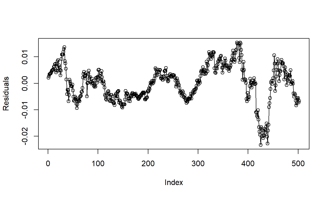
Figure 8.7: Residuals from a Quadratic Trend in Time Model of the Hong Kong Exchange Rates.
R Code to Produce Figure 8.7
Further evidence of these patterns is in the table of autocorrelations in Table 8.6. Here, we see large residual autocorrelations that do not decrease quickly as the lag \(k\) increases. A similar pattern is also evident for the original series, EXHKUS. This confirms the nonstationarity that we observed in Section 7.2.
As an alternative transform, we differenced the series, producing DIFFHKUS. This differenced series has a standard deviation of \(s_{DIFF}=0.0020\), suggesting that it is more stable than the original series or the residuals from the quadratic trend in time model. Table 8.6 presents the autocorrelations from the differenced series, indicating mild patterns. However, these autocorrelations are still significantly different from zero. For \(T=501\) differences, we may use as an approximate standard error for autocorrelations \(1/\sqrt{501}\approx 0.0447.\) With this, we see that the lag 2 autocorrelation is \(0.151/0.0447\approx 3.38\) standard errors below zero, which is statistically significant. This suggests introducing another model to take advantage of the information in the time series patterns.
Table 8.6. Autocorrelations of Hong Kong Exchange Rates
\[ \small{ \begin{array}{l|cccccccccc} \hline \text{Lag }& 1 & 2 & 3 & 4 & 5 & 6 & 7 & 8 & 9 & 10 \\ \hline \text{Residuals from the} & 0.958 & 0.910 & 0.876 & 0.847 & 0.819 & 0.783 & 0.748 & 0.711 & 0.677 & 0.636 \\ \ \ \text{Quadratic Model} & & & & & & & & & & \\ \text{EXHKUS} & 0.988 & 0.975 & 0.963 & 0.952 & 0.942 & 0.930 & 0.919 & 0.907 & 0.895 & 0.882 \\ \ \ \text{(Original Series)} & & & & & & & & & & \\ \text{DIFFHKUS} & 0.078 & -0.151 & -0.038 & -0.001 & 0.095 & -0.005 & 0.051 & -0.012 & 0.084 & -0.001 \\ \hline \end{array} } \]
R Code to Produce Table 8.6
Model Selection and Partial Autocorrelations
For all stationary autoregressive models, it can be shown that the absolute values of the autocorrelations become small as the lag \(k\) increases. In the case that the autocorrelations decrease approximately like a geometric series, an \(AR\)(1) model may be identified. Unfortunately, for other types of autoregressive series, the rules of thumb for identifying the series from the autocorrelations become more cloudy. One device that is useful for identifying the order of an autoregressive series is the partial autocorrelation function.
Just like autocorrelations, we now define a partial autocorrelation at a specific lag \(k\). Consider the model equation \[ y_t=\beta_{0,k}+\beta_{1,k} y_{t-1}+\ldots+\beta_{k,k} y_{t-k} + \varepsilon_t. \] Here, {\(\varepsilon_t\)} is a stationary error that may or may not be a white noise process. The second subscript on the \(\beta\)’s, “\(,k\)”, is there to remind us that the value of each \(\beta\) may change when the order of the model, \(k\), changes. With this model specification, we can interpret \(\beta_{k,k}\) as the correlation between \(y_t\) and \(y_{t-k}\) after the effects of the intervening variables, \(y_{t-1},\ldots,y_{t-k+1}\), have been removed. This is the same idea as the partial correlation coefficient, introduced in Section 4.4. Estimates of partial correlation coefficients, \(b_{k,k}\), can then be calculated using conditional least squares or other techniques. As with other correlations, we may use \(1/\sqrt{T}\) as an approximate standard error for detecting significant differences from zero.
Partial autocorrelations are used in model identification in the following way. First calculate the first several estimates, \(b_{1,1},b_{2,2},b_{3,3}\), and so on. Then, choose the order of the autoregressive model to be the largest \(k\) so that the estimate \(b_{k,k}\) is significantly different from zero.
To see how this applies in the Hong Kong Exchange Rate example, recall that the approximate standard error for correlations is \(1/\sqrt{501}\approx 0.0447\). Table 8.7 provides the first ten partial autocorrelations for the rates and for their differences. Using twice the standard error as our cut-off rule, we see that the second partial autocorrelation of the differences exceeds \(2\times 0.0447=0.0894\) in absolute value. This would suggest using an \(AR(2)\) as a tentative first model choice. Alternatively, the reader may wish to argue that because the fifth and ninth partial autocorrelations are also statistically significant, suggesting a more complex \(AR(5)\) or \(AR(9)\) would be more appropriate. The philosophy is to “use the simplest model possible, but no simpler.” We prefer to employ simpler models and thus fit these first and then test to see whether or not they capture the important aspects of the data.
Finally, you may be interested to see what happens to partial autocorrelations calculated on a non-stationary series. Table 8.7 provides partial autocorrelations for the original series (EXHKUS). Note how large the first partial autocorrelation is. That is, yet another way of identifying a series as nonstationary is to examine the partial autocorrelation function and look for a large lag one partial autocorrelation.
Table 8.7. Partial Autocorrelations of EXHKUS and DIFFHKUS
\[ \small{ \begin{array}{l|cccccccccc} \hline \text{Lag} & 1 & 2 & 3 & 4 & 5 & 6 & 7 & 8 & 9 & 10 \\ \hline \text{EXHKUS} & 0.988 & -0.034 & 0.051 & 0.019 & -0.001 & -0.023 & 0.010 & -0.047 & -0.013 & -0.049 \\ \text{DIFFHKUS} & 0.078 & -0.158 & -0.013 & -0.021 & 0.092 & -0.026 & 0.085 & -0.027 & 0.117 & -0.036 \\ \hline \end{array} } \]
R Code to Produce Table 8.7
Residual Checking
Having identified and fit a model, residual checking is still an important part of determining a model’s validity. For the \(ARMA(p,q)\) model, we compute fitted values as
\[\begin{equation} \widehat{y}_t = b_0 + b_1 y_{t-1} + \ldots + b_p y_{t-p} - \widehat{\theta}_1 e_{t-1}- \ldots - \widehat{\theta }_q e_{t-q}. \tag{8.13} \end{equation}\] Here, \(\widehat{\theta}_1, \ldots, \widehat{\theta}_q\) are estimates of \(\theta_1,\ldots, \theta_q\). The residuals may be computed in the usual fashion, that is, as \(e_t=y_t-\widehat{y}_t\). Without further approximations, note that the initial residuals are missing because fitted values before time \(t=\max (p,q)\) can not be calculated using equation (8.13). To check for patterns, use the devices described in Section 8.3, such as the control chart to check for stationarity and the autocorrelation function to check for lagged variable relationships.
Residual Autocorrelation
Residuals from the fitted model should resemble white noise and hence, display few discernible patterns. In particular, we expect \(r_k(e)\), the lag \(k\) autocorrelation of residuals, to be approximately zero. To assess this, we have that \(se\left( r_k(e) \right) \approx 1/\sqrt{T}\). More precisely, MacLeod (1977, 1978) has given approximations for a broad class of \(ARMA\) models. It turns out that the \(1/\sqrt{T}\) can be improved for small values of \(k\). (These improved values can be seen in the output of most statistical packages.) The improvement depends on the model that is being fit. To illustrate, suppose that an \(AR(1)\) model with autoregressive parameter \(\beta_1\) is fit to the data. Then, the approximate standard error of the lag one residual autocorrelation is \(|\beta_1|/\sqrt{T}\) . This standard error can be much smaller than \(1/\sqrt{T}\), depending on the value of \(\beta_1\).
Testing Several Lags
To test whether there is significant residual autocorrelation at a specific lag \(k\), we use \(r_k(e) /se\left( r_k(e) \right)\). Further, to check whether residuals resemble a white noise process, we might test whether \(r_k(e)\) is close to zero for several values of \(k\). To test whether the first \(K\) residual autocorrelation are zero, use the Box and Pierce (1970) chi-square statistic \[ Q_{BP} = T \sum_{k=1}^{K} r_k \left( e \right)^2. \] Here, \(K\) is an integer that is user-specified. If there is no real autocorrelation, then we expect \(Q_{BP}\) to be small; more precisely, Box and Pierce showed that \(Q_{BP}\) follows an approximate \(\chi^2\) distribution with \(df=K-(number~of~linear~parameters)\). For an \(ARMA(p,q)\) model, the number of linear parameters is \(1+p+q.\) Another widely used statistic is \[ Q_{LB}=T(T+2)\sum_{k=1}^{K}\frac{r_k \left( e\right)^2}{T-k}. \]
due to Ljung and Box (1978). This statistic performs better in small samples than the \(BP\) statistic. Under the hypothesis of no residual autocorrelation, \(Q_{LB}\) follows the same \(\chi^2\) distribution as \(Q_{BP}\). Thus, for each statistic, we reject \(H_{0}\): No Residual Autocorrelation if the statistic exceeds \(chi\)-value, a \(1-\alpha\) percentile from a \(\chi^2\) distribution. A convenient rule of thumb is to use \(chi\)-value = 1.5 \(df.\)
Example: Hong Kong Exchange Rate - Continued. Two models were fit, the \(ARIMA(2,1,0)\) and the \(ARIMA(0,1,2)\); these are the \(AR(2)\) and \(MA(2)\) models after taking differences. Using {\(y_t\)} for the differences, the estimated \(AR(2)\) model is: \[ \begin{array}{clllrllll} \widehat{y}_t & = & 0.0000317 & + & 0.0900 & y_{t-1} & - & 0.158 & y_{t-2} \\ {\small t-statistic} & & {\small [0.37]} & & {\small [2.03]} & & & {\small [-3.57]} & \end{array} \] with a residual standard error of \(s=0.00193.\) The estimated \(MA(2)\) is: \[ \begin{array}{clllrllll} \widehat{y}_t & = & 0.0000297 & - & 0.0920 & e_{t-1} & + & 0.162 & e_{t-2} \\ {\small t-statistic} & & {\small [0.37]} & &{\small [-2.08]} & & & {\small [3.66]} & \end{array} \] with the same residual standard error of \(s=0.00193.\) These statistics indicate that the models are roughly comparable. The Ljung-Box statistic in Table 8.8 also indicates a great deal of similarity for the models.
Table 8.8. Ljung-Box Statistics \(Q_{LB}\) for Hong Kong Exchange Rate Models
\[ \small{ \begin{array}{l|ccccc} \hline &&& \text{Lag }K \\ \text{Model} & 2 & 4 & 6 & 8 & 10 \\ \hline AR(2) & 0.0065 & 0.5674 & 6.3496 & 10.4539 & 16.3258 \\ MA(2) & 0.0110 & 0.2872 & 6.6557 & 11.3361 & 17.6882 \\ \hline \end{array} } \]
R Code to Produce Table 8.8
The fitted \(MA\)(2) and \(AR\)(2) models are roughly similar. We present the \(AR\)(2) model for forecasting only because autoregressive models are typically easier to interpret. Figure 8.8} summarizes the predictions, calculated for ten days. Note the widening forecast intervals, typical of forecasts for nonstationary series.
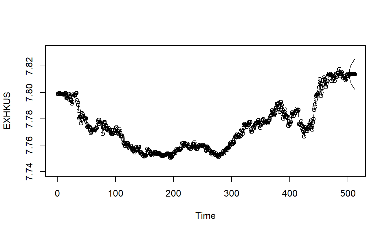
Figure 8.8: Ten Day Forecasts and Forecast Intervals of the Hong Kong Exchange Rates. Forecasts are based on the \(ARIMA(2,1,0)\) model.
R Code to Produce Figure 8.8
8.7 Further Reading and References
The classic book-long introduction to Box-Jenkins time series is Box, Jenkins and Reinsel (1994).
Chapter References
- Abraham, Bovas and Johannes Ledolter (1983). Statistical Methods for Forecasting. John Wiley & Sons, New York.
- Box, George E. P., Gwilym M. Jenkins and Gregory C. Reinsel (1994). Time Series Analysis: Forecasting and Control, Third Edition, Prentice-Hall, Englewood Cliffs, New Jersey.
- Box, George E. P., and D. A. Pierce (1970). Distribution of residual autocorrelations in autoregressive moving average time series models. Journal of the American Statistical Association 65, 1509-1526.
- Chan, Wai-Sum and Siu-Hang Li (2007). The Lee-Carter model for forecasting mortality, revisited. North American Actuarial Journal 11(1), 68-89.
- Lee, Ronald D. and Lawrence R. Carter (1992). Modelling and forecasting U.S. mortality. Journal of the American Statistical Association 87, 659-671.
- Ljung, G. M. and George E. P. Box (1978). On a measure of lack of fit in time series models. Biometrika 65, 297-303.
- MacLeod, A. I. (1977). Improved Box-Jenkins estimators. Biometrika 64, 531-534.
- MacLeod, A. I. (1978). On the distribution of residual autocorrelations in Box-Jenkins models. Journal of the Royal Statistical Society B 40, 296-302.
- Miller, Robert B. and Dean W. Wichern (1977). Intermediate Business Statistics: Analysis of Variance, Regression and Time Series. Holt, Rinehart and Winston, New York.
- Roberts, Harry V. (1991). Data Analysis for Managers with MINITAB. Scientific Press, South San Francisco, CA.
8.8 Exercises
8.1. A mutual fund has provided investment yield rates for five consecutive years as follows:
\[ \begin{array}{l|ccccc} \hline \text{Year} & 1 & 2 & 3 & 4 & 5 \\ \hline \text{Yield} & 0.09 & 0.08 & 0.09 & 0.12 & -0.03 \\ \hline \end{array} \]
Determine \(r_1\) and \(r_2\), the lag 1 and lag 2 autocorrelation coefficients.
8.2. The Durbin-Watson statistic is designed to detect autocorrelation and is defined by: \[ DW = \frac {\sum_{t=2}^T (y_t - y_{t-1})^2} {\sum_{t=1}^T (y_t - \bar{y})^2}. \]
Derive the approximate relationship between \(DW\) and the lag 1 autocorrelation coefficient \(r_1\).
Suppose that \(r_1 = 0.4\). What is the approximate value of \(DW\)?
8.3. Consider the Chapter 2 linear regression model formulas with \(y_{t-1}\) in place of \(x_t\), for \(t=2, \ldots, T\).
Provide an exact expression for \(b_1\).
Provide an exact expression for \(b_0\).
Show that \(b_0 \approx \bar{y} (1-r_1)\).
8.4. Begin with the \(AR\)(1) model as in equation (8.1).
Take variances of each side of equation (8.1) to show that \(\sigma_y^2(1-\beta_1^2) = \sigma^2,\) where \(\sigma_y^2 = \mathrm{Var}~y_t\) and \(\sigma^2 = \mathrm{Var}~\varepsilon_t\).
Show that \(\mathrm{Cov}(y_t,y_{t-1}) = \beta_1 \sigma_y^2.\)
Show that \(\mathrm{Cov}(y_t,y_{t-k}) = \beta_1^k \sigma_y^2.\)
Use part (c) to establish equation (8.2).
8.5. Consider forecasting with the \(AR\)(1) model.
Use the forecasting chain rule in equation (8.4) to show \[ y_{T+k}-\widehat{y}_{T+k} \approx \varepsilon_{T+k} + \beta_1 \varepsilon_{T+k-1} + \cdots + \beta_1^{k-1} \varepsilon_{T+1}. \]
From part (a), show that the approximate variance of the forecast error is \(\sigma^2 \sum_{l=0}^{k-1} \beta_1^{2l}.\)
8.6. These data consist of the 503 daily returns for the calendar years 2005 and 2006 of the Standard and Poor’s (S&P) value weighted index. (The data file contains additional years - this exercise uses only 2005 and 2006 data.) Each year, there are about 250 days on which the exchange is open and stocks were traded - on weekends and holidays it is closed. There are several indices to measure the market’s overall performance. The value weighted index is created by assuming that the amount invested in each stock is proportional to its market capitalization. Here, the market capitalization is simply the beginning price per share times the number of outstanding shares. An alternative is the equally weighted index, created by taking a simple average of the closing, or last, price of stocks that form the S&P on that trading day.
Financial economic theory states that if the market were predictable, many investors would attempt to take advantage of these predictions, thus forcing unpredictability. For example, suppose a statistical model reliably predicted mutual fund A to increase two-fold over the next 18 months. Then, the no arbitrage principle in financial economics states that several alert investors, armed with information from the statistical model, would bid to buy mutual fund A, thus causing the price to increase because demand is increasing. These alert investors would continue to purchase until the price of mutual fund A rose to the point where the return was equivalent to other investment opportunities in the same risk class. Thus, any advantages produced by the statistical model would disappear rapidly, thus eliminating this advantage.
Thus, financial economic theory states that for liquid markets such as stocks represented through the S&P index there should be no detectable patterns, resulting in a white noise process. In practice, it has been found that cost of buying and selling equities (called transactions costs) are large enough so as to prevent us from taking advantage of these slight tendencies in the swings of the market. This illustrates a point known as statistically significant but not practically important. This is not to suggest that statistics is not practical (heavens forbid!). Instead, statistics in and of itself does not explicitly recognize factors, such as economic, psychological and so on, that may be extremely important in any given situation. It is up to the analyst to interpret the statistical analysis in light of these factors.
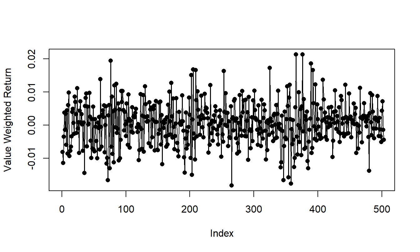
Figure 8.9: Time Series Plot of the S & P Daily Market Return, 2005-2006.
R Code to Produce Figure 8.9
The time series plot in Figure 8.9 gives a preliminary idea of the characteristics of the sequence. Comment on the stationarity of the sequence.
Calculate summary statistics of the sequence. Suppose that you assume a white noise model for the the sequence. Compute 1, 2 and 3 step ahead forecasts for the daily returns for the first three trading days of 2007.
Calculate the autocorrelations for the lags 1 through 10. Do you detect any autocorrelations that are statistically significantly different from zero?