Chapter 19 Claims Triangles
Chapter Preview. This chapter introduces a classic actuarial reserving problem that is encountered extensively in property and casualty as well as health insurance. The data are presented in a triangular format to emphasize their longitudinal and censored nature. This chapter explains how such data arise naturally and introduces regression methods to address the actuarial reserving problem.
19.1 Introduction
In many types of insurance, little time elapses between the event of a claim, notification to an insurance company and payment to beneficiaries. For example, in life insurance notification and benefit payments typically occurs within two weeks of an insured’s death. However, for other lines of insurance, times from claim occurrence to the final payment can be much longer, taking months and even years. To introduce this situation, this section describes the evolution of a claim, introduces summary measures used by insurers and then describes the prevailing deterministic method for forecasting claims, the chain ladder method.
19.1.1 Claims Evolution
For example, suppose that you become injured in an automobile accident covered by insurance. It can take months for the injury to heal and all of the medical care payments to become known and paid by the insurance company. Moreover, disputes may arise among you, other parties to the accident, your insurer and insurer(s) of other parties, thus lengthening the time until claims are settled and paid. When claims take a long time to develop, an insurer’s claim obligations may be incurred in one accounting period but not paid until a later accounting period. In the example of your accident, the insurer is aware that a claim has occurred and may have even made some payments in the current accounting period. Future payment amounts are unknown by the end of the current accounting period but the insurer wishes to make an accurate forecast of future obligations to set aside a fair amount of money of future obligations, known as a reserve. The insurer’s objective is to use current claim information to predict the timing and amount of future claim payments.
To set terminology, it is helpful to follow the timeline of a claim as it develops. In Figure 19.1, the claim occurs at time \(t_1\) and the insuring company is notified at time \(t_3\). There can be a long gap between occurrence and notification such that a valuation date (\(t_2\)) may occur within this gap. Here, \(t_2\) is the time when the obligations are valued which is typically but not always at the end of a company financial reporting period. In this case, the claim is said to be incurred but not reported at this valuation date.
After claim notification, there may one or more loss payments. Not all of the payments may be made by the next valuation date (\(t_4\)). As the claim develops, eventually the company deems its financial obligations on the claim to be resolved and declares the claim “closed.” However, it is possible that new facts arise and the claim must be re-opened, giving rise to additional loss payments prior to being closed again.
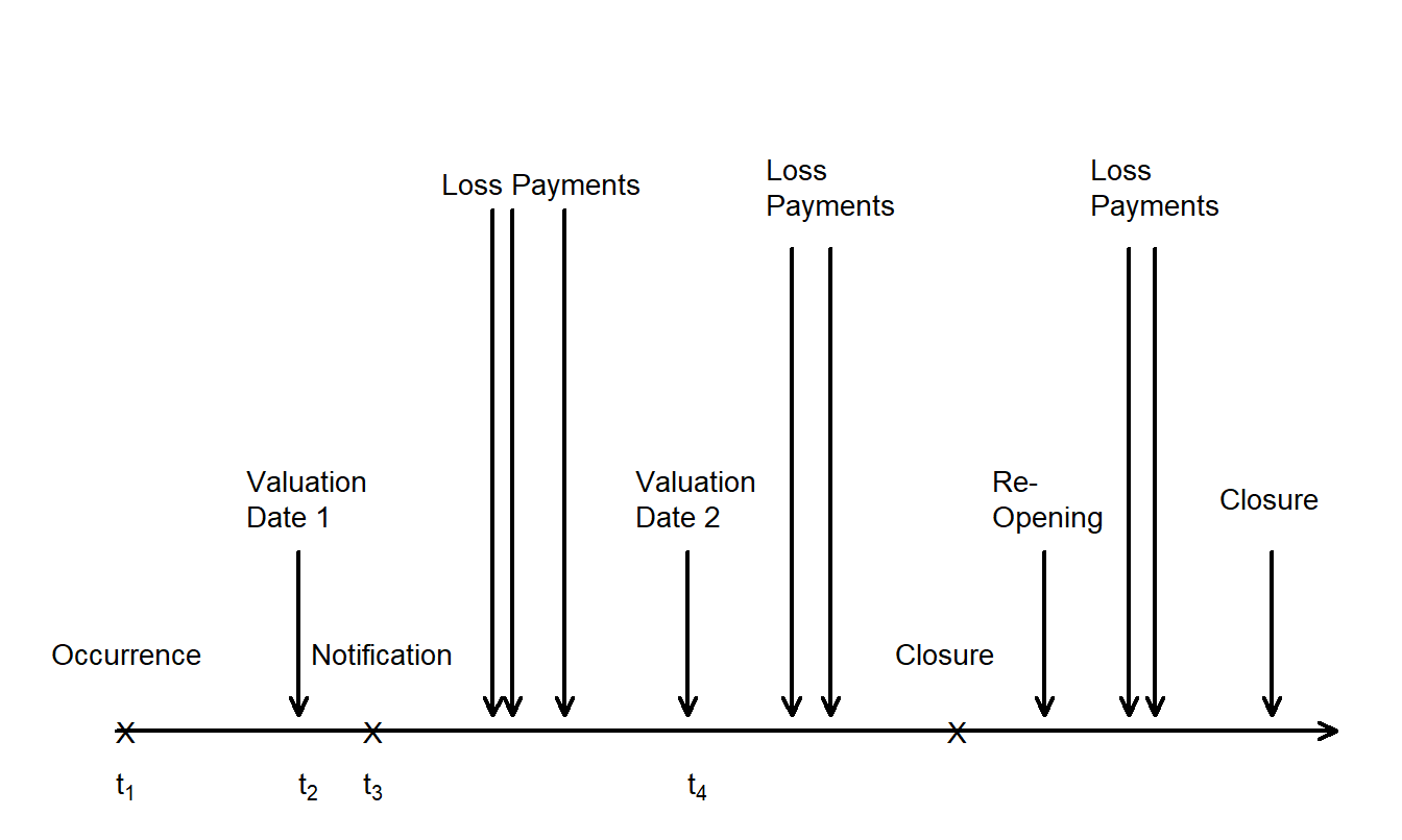
Figure 19.1: Timeline of Claim Development.
19.1.2 Claims Triangles
Insurers do not typically model the evolution of each claim and then sum them (as is done on a policy basis in life insurance). Instead, portfolios of claims are summarized at each valuation date; it is these summaries upon which forecasts of outstanding claims are based.
Specifically, let \(i\) represent the year in which a claim has been incurred and \(j\) represent the number of years from incurral to the time when the payment is made, the “development” (or “delay”) year. Thus, \(y_{ij}\) represents the sum of payment amounts in the \(i\)th incurral and \(j\)th development year. Here, “year” refers to the accounting period - in subsequent examples, you will see that we often use month, quarter or other fixed period. Table 19.1 shows the information that actuaries typically confront.
Table 19.1. Classic Claims Run-Off Triangle
\[ \small{ \begin{array}{c|ccccc} \hline \text{Incurral} & \text{Development Year }&(j) \\ \text{Year }(i) & 1& 2& 3&4&5 \\ \hline 1 & y_{11} & y_{12} & y_{13} & y_{14} & y_{15} \\ 2 & y_{21} & y_{22} & y_{23} & y_{24} & . \\ 3 & y_{31} & y_{32} & y_{33} & . & . \\ 4 & y_{41} & y_{42} & . &. & . \\ 5 & y_{51} & . & . &. & . \\ \hline \end{array} } \]
The term “claims triangle” is evident from Table 19.1. We observe data in the upper left-hand triangle, \(y_{ij}, i=1,\ldots, 5, j=1, \ldots,6-i\). The goal is “to complete the triangle,” that is, to forecast values in the lower right-hand triangle (\(y_{ij}, i=2,\ldots, 5, j=7-i, \ldots,5\)). For example, the most recent incurral year is \(i=5\) for which we have only one year of claims experience, \(y_{51}\). The other values, \(y_{5j}, j=2, \ldots,5\), are unknown at the valuation date. In some situations, it is also of interest to forecast claims in development years six and beyond.
Table 19.1 underscores the fact that data are both longitudinal and censored. This is the key point regarding statistical modeling assumptions. In applications, the observations can vary significantly depending on the type and purpose. Each element of the triangle may represent actual payments by the insurance company, known as “incremental payments,” or the “cumulative” sum of payments since development. For some lines of business, estimates of the outstanding payments are available on a claim-by-claim basis, known as “case estimates.” Here, triangle elements may represent incurred claims in lieu of paid claims. That is, an incurred claim is the paid amount plus the reserve. Because case estimates are revised as new information about a claim comes in, it is not uncommon for incurred payments to be negative. Further, even paid incremental payments can be negative due to reinsurance or recovery from other parties of claims amounts. (Many insurers will write checks to pay claimants quickly upon the occurrence of an accident and later be reimbursed by another party responsible for the accident.) Claims triangle data can also be in the form of the number of claim notifications. This type of data is particularly useful for estimating “incurred but not reported” reserves.
Example: Singapore Property Damage. Table 19.2 reports incremental payments from a portfolio of automobile policies for a Singapore property and casualty (general) insurer. Here, payments are for third party property damage from comprehensive auto insurance policies. All payments have been deflated using a Singaporean consumer price index, so they are in constant dollars. The data are for policies with coverages from 1997-2001, inclusive. Table 19.2 also provides the premiums for these policies (in thousands of Singaporean dollars) to provide a sense of the insurer’s increasing exposure to potential claim obligations.
Table 19.2. Singapore Incremental Payments
\[ \small{ \begin{array}{lr|rrrrr} \hline \text{Incurral} & \text{Premium} &\text{ Development} & \text{Year} \\ \text{ Year } & \text{(in thousands)} & 1 & 2 & 3 & 4 & 5 \\ \hline 1997 & 32,691 & 1,188,675 & 2,257,909 & 695,237 & 166,812 & 92,129 \\ 1998 & 33,425 & 1,235,402 & 3,250,013 & 649,928 & 211,344 & . \\ 1999 & 34,849 & 2,209,850 & 3,718,695 & 818,367 & . & . \\ 2000 & 37,011 & 2,662,546 & 3,487,034 & . & . & . \\ 2001 & 40,152 & 2,457,265 & . & . & . & . \\ \hline \end{array} } \]
R Code to Produce Table 19.2
19.1.3 Chain Ladder Method
To introduce the basic chain ladder method, we continue to work in the context of the Singapore property damage example. Table 19.3 shows the same payments as Table 19.2 but in cumulative rather than incremental form. Let \(S_{ij} = y_{i1} + \cdots + y_{ij}\) denote cumulative claims.
Table 19.3. Singapore Cumulative Payments with Chain Ladder Estimates
\[ \scriptsize{ \begin{array}{lllrrrr|r|c} \hline \hline &&&&&&&&\text{Ultimate}\\ &&&&&&&& \text{Loss} \\ \text{Incurral} &&\text{Development}& \text{Year} & &&&&\text{Ratio} \\ \text{Year} & \text{ Premium} &~~~~~~~~1 & 2~~~ & 3~~~& 4~~~& 5~~~& \text{ Reserve} & (\%) \\ \hline 1997 & 32,691 & 1,188,675 & 3,446,584 & 4,141,821 & 4,308,633 & 4,400,762 & & 13.5 \\ 1998 & 33,425 & 1,235,402 & 4,485,415 & 5,135,343 & 5,346,687 & {\bf 5,461,012} & 114,325 & 16.3 \\ 1999 & 34,849 & 2,209,850 & 5,928,544 & 6,746,912 & {\bf 7,021,930} & {\bf 7,172,075} & 425,163 & 20.6 \\ 2000 & 37,011 & 2,662,546 & 6,149,580 & {\bf 7,109,486} & {\bf 7,399,283} & {\bf 7,557,497} & 1,407,917 & 20.4 \\ 2001 & 40,152 & 2,457,265 &{\bf 6,738,898} & {\bf 7,790,792} & {\bf 8,108,361} & {\bf 8,281,737} & 5,824,471 & 20.6 \\ \hline \text{Total} &\text{Reserve} & & & & &&7,771,877 \\ Chain & Ladder& Factors & 2.742 & 1.156 & 1.041 & 1.021 & \\ \hline \hline \end{array} } \]
The chain ladder factor for the \(j\)th development year is calculated by taking the ratio of the sum of claims over all incurral years for the \(j\)th development year divided by the sum of the same incurral year payments for the \(j-1^{st}\) development year. Using notation, we have \[ CL_j = \frac {\sum_{i=1}^{6-j} S_{ij}}{\sum_{i=1}^{6-j} S_{i,j-1}}. \] For example, \(CL_5 = 4,400,762/4,308,633 = 1.021\) and \(CL_4 = (5,346,687+4,308,633)/(5,135,343+4,141,821)= 1.041\).
Bold numbers are forecasts calculated recursively using the chain ladder factors and \(\widehat{S}_{i,j} = CL_{j} \times \widehat{S}_{i,j-1}.\) The recursion starts when the value of the cumulative payment is known so that \(\widehat{S}_{ij}=S_{ij}\). For example, for incurral year 2, \(\widehat{S}_{25} = CL_5 \times S_{24} = (1.021)(5,346,687)=5,461,012\). For incurral year 3, \(\widehat{S}_{34} = CL_4 \times S_{33} = (1.041)(6,746,912)=7,021,930\) and \(\widehat{S}_{35} = CL_5 \times \widehat{S}_{34} = (1.021)(7,021,930)=7,172,075\). Alternatively, one can go directly to the last development year and use \(\widehat{S}_{35} = CL_5 \times \widehat{S}_{34} = CL_5 \times CL_4 \times S_{33} = (1.041)(1.021)(6,746,912)=7,172,075.\)
In Table 19.3, the reserve is the ultimate forecast amount minus the most recent cumulative paid claim. The ultimate loss ratio is the ratio of the forecast of cumulative claims in the last development year (5) to premiums paid (expressed as a percentage, recall that premiums are in thousands).
19.2 Regression Using Functions of Time as Explanatory Variables
The chain ladder method is an important tool that actuaries use extensively when forecasting claims. It is typically presented as deterministic, as in Section 19.1.3. Alternative stochastic models for claim forecasting have two primary advantages.
- By explicitly modeling the distribution of claims, estimates for the uncertainty of the reserve forecasts can be made.
- There are many variations of chain ladder techniques available because they are applied in many different situations. As we have seen in Chapter 5, stochastic methods feature a disciplined way of model selection that can help determine the most appropriate model for a given set of data.
As we will see, one need not make a choice between using the chain ladder method and a stochastic model. The Section 19.2.3 overdisperse Poisson model and the Section 19.3.1 Mack model both yield point forecasts that are equal to chain ladder forecasts.
19.2.1 Lognormal Model
Our starting point is the lognormal model for incremental claims. That is, we consider a two factor model of the form
\[\begin{equation} \ln y_{ij} = \mu + \alpha_i + \tau_j + \varepsilon_{ij}, \tag{19.1} \end{equation}\] where \(\{ \alpha_i \}\) are parameters for the incurral year factor and \(\{ \tau_j \}\) are parameters for the development year factor. A regression model with two factors was introduced in Section 4.4. Recall that we require constraints on the factor parameters for estimability such as \(\sum_i \alpha_i = 0\) and \(\sum_j \tau_j= 0\). Assuming normality of \(\{\varepsilon_{ij} \}\) gives rise to the lognormal specification for the incremental claims \(y_{ij}\).
Example: Singapore Third Party Injury. Table 19.4 reports payments from a portfolio of automobile policies for a Singapore property and casualty (general) insurer. Payments, deflated for inflation, are for third party injury from comprehensive insurance policies. The data are for policies with coverages from 1993-2001, inclusive.
In automobile insurance, it typically takes longer to settle and pay injury compared to property damage claims. Thus, the number of development years, “the run-off,” is longer in Table 19.4 than Table 19.2. Table 19.4 also shows a lack of stability of injury payments that Figure 19.2 helps us visualize. The left-hand panel shows trend lines by development for each incurral year. The right-hand panel presents box plots of logarithmic payments for each development year. This display shows that payments tend to rise for the first two development periods (\(j=1,2\)), reach a peak at the third period (\(j=3\)) and decline thereafter.
Table 19.4. Singapore Incremental Injury Payments, 1993-2001
\[ \small{ \begin{array}{c|rrrrrrrrr} \hline \text{Incurral}&\text{Development} &\text{Year} \\ \text{Year} & 1 & 2 &3 &4 & 5 & 6 & 7 & 8 & 9 \\ \hline 1993 & 14,695 & 205,515 & 118,686 & 416,286 & 93,544 & 185,043 & 37,750 & 0 &14,086 \\ 1994 & 153,615 & 467,722 & 645,513 & 421,896 & 146,576 & 96,470 & 27,765 &38,017 & . \\ 1995 & 24,741 & 547,862 & 754,475 & 417,573 & 156,596 & 55,155 & 36,984 & . & . \\ 1996 & 68,630 & 188,627 & 492,306 & 179,249 & 34,062 & 443,436 & . & . & . \\ 1997 & 29,177 & 364,672 & 437,507 & 385,571 & 529,319 & . & . & . & . \\ 1998 & 40,430 & 241,809 & 678,541 & 528,026 & . & . & . & . & . \\ 1999 & 45,125 & 372,935 & 704,168 & . & . & . & . & . & . \\ 2000 & 21,695 & 158,005 & . & . & . & . & . & . & . \\ 2001 & 6,626 & . & . & . & . & . & . & . & . \\ \hline \hline \end{array} } \]
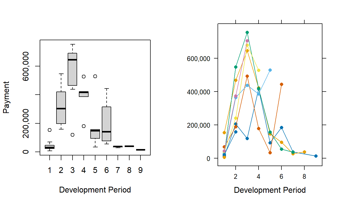
Figure 19.2: Singapore Incremental Injury Payments. The left-hand panel shows payments by development year with each line connecting payments from the same incurral year. The right-hand panel shows the distribution of logarithmic payments for each development year.
R Code to Produce Figure 19.2
The lognormal model based on equation (19.1) was fit to these data. Not surprisingly, both factors incurral and development year were statistically significant. The coefficient of determination from the fit is \(R^2 = 73.3 \%\). A \(qq\) plot (not presented here) showed reasonable agreement with the assumption of normality. Fitted values from the model, after exponentiation to convert back to dollars, appear in Figure 19.3. This figure seems to capture the payment patterns that appear in the left-hand panel of Figure 19.2. Note that the fitted values for the unobserved portion of the triangle are forecasts.
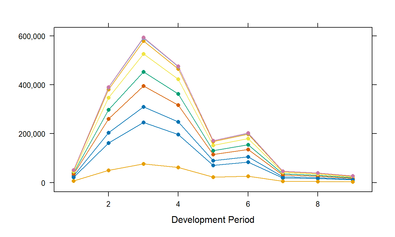
Figure 19.3: Fitted Values for the Singapore Incremental Injury Payments. These estimates are based on the two factor lognormal model.
R Code to Produce Figure 19.3
19.2.2 Hoerl Curve
The systematic component of equation (19.1) can be easily modified. One possibility is the so-called “Hoerl curve,” leading to the model equation
\[\begin{equation} \ln y_{ij} = \mu + \alpha_i + \beta_i \ln (j) + \gamma_i \times j + \varepsilon_{ij} . \tag{19.2} \end{equation}\] An advantage of treating development time \(j\) as a continuous covariate is that extrapolation is possible beyond the range of development times observed. As a variation, England and Verrall (2002) suggest allowing the first few development years to have their own levels and imposing the same run-off pattern for all incurral years (\(\beta_i = \beta\), \(\gamma_i = \gamma\)).
Example: Singapore Third Party Injury - Continued. The basic model from equation (19.2) fit well, the coefficient of determination is \(R^2 = 87.8 \%\). We also examined a simpler model based on the equation \[\begin{equation} \ln y_{ij} = \mu + \alpha_i + \beta \ln (j) + \gamma \times j + \varepsilon_{ij} . \tag{19.3} \end{equation}\] This simpler model did not fit the data as well as the more complete Hoerl model from equation (19.2), having \(R^2 = 78.6\%\). However, a partial \(F\) test established that the additional parameters were not statistically significant and so the simpler model in equation (19.3) is preferred.
Based on the simpler model, fitted values are displayed in Figure 19.4. This figure displays the geometrically declining fitted values beginning in the fourth development period.
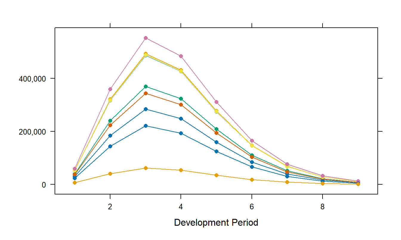
Figure 19.4: Fitted Values from the Reduced Hoerl Model in Equation (19.3).
R Code to Produce Figure 19.4
19.2.3 Poisson Models
A drawback of the lognormal model is that the predictions produced by it do not replicate the traditional chain-ladder estimates. This section introduces the overdisperse Poisson model that does have this desirable feature.
To begin, from equation (19.1), we may write \[ \mathrm{E}~ y_{ij} = \exp(\eta_{i,j})~~ \mathrm{E}~ e^{\varepsilon} \] where the systematic component is \(\eta_{i,j} = \mu + \alpha_i + \tau_j\). This is a model with a logarithmic link function (that is, \(\ln \mathrm{E}~y = \eta\)). Instead of using the lognormal distribution for \(y\), this section assumes that \(y\) follows an overdisperse Poisson with variance function \[ \mathrm{Var}~ y_{ij} = \phi \exp(\eta_{i,j}). \] Note that we have absorbed the scalar \(\mathrm{E}~ e^{\varepsilon}\) into the overdispersion parameter \(\phi\).
We introduced overdisperse Poisson models in Section 12.3. Thus, this model can be estimated with standard statistical software and, as with the lognormal model, forecasts readily produced. It can be shown that the forecasts produced by the overdisperse Poisson are equivalent to the deterministic chain ladder forecasts. See, for example Taylor (2000) or Wüthrich and Merz (2008) for a proof. Not only does this give us a mechanism to quantify the uncertainty associated with chain ladder forecasts, we can also use standard statistical software to compute these estimates.
Example: Singapore Third Party Injury - Continued. The overdisperse Poisson model was fit to the Singapore injury payments data. Standard statistical software was use to compute parameter estimates, using techniques described in Section 12.3. Figure 19.5 summarizes the forecasts from these models. This figure shows cumulative, not incremental, payments, marked with opaque plotting symbols in the figure. Forecasts of incremental payments were produced and then summed to get the cumulative payment forecasts in Figure 19.5; these are marked with the open plotting symbols. The reader is invited to check that these forecasts are identical to those produced by the deterministic chain ladder method up to the eight development year. Here, the value of zero for the first incurral year causes small differences between the Poisson model and chain ladder forecasts.
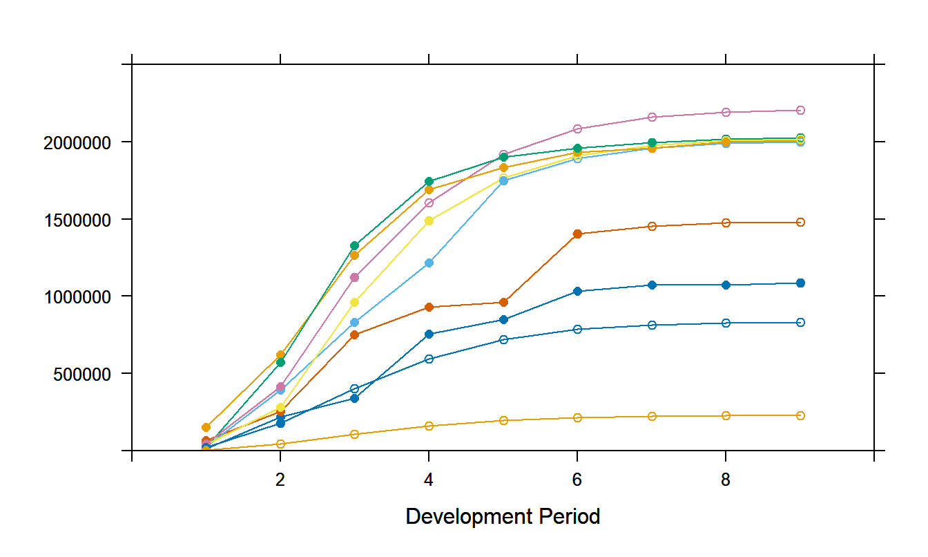
Figure 19.5: Actual and Forecast Values for the Singapore Cumulative Injury Payments. Actual values are denoted with an opaque plotting symbol. Chain ladder forecasts, from an overdisperse Poisson model, are denoted with an open plotting symbol.
R Code to Produce Figure 19.5
19.3 Using Past Developments
As with autoregressive models, one can use prior history to forecast payments. What is prior history? In the claim triangle set-up in Table 19.1, there are two dimensions of time: incurral year and development year. Most models focus on using prior development (“\(j\)”) for forecasting. By focusing on prior development experience, we allow ourselves the flexibility to our model cumulative (\(S_{ij}\)) or incremental (\(y_{ij}\)) payments. As we learned in our Chapters 7 and 8 study of time series, it is useful to be able to model both a series (\(S_{ij}\)) and its changes (\(y_{ij} = S_{ij}-S_{i,j-1}\)).
19.3.1 Mack Model
The model put forward by Mack (1993) specifies the first two conditional moments of cumulative payments and uses generalized least squares to fit the model. Under this stochastic specification, traditional chain ladder forecasts are produced.
Specifically, we assume
\[\begin{equation} \mathrm{E} \left( S_{i,j} | S_{i,j-1} \right) = \nu_j S_{i,j-1} \tag{19.4} \end{equation}\] and \[\begin{equation} \mathrm{Var} \left( S_{i,j} | S_{i,j-1} \right) = \sigma^2_j , S_{i,j-1} \tag{19.5} \end{equation}\] where \(\nu_j\) and \(\sigma^2_j\) are model parameters.
The mean parameters, \(\nu_j\), are determined through generalized least squares by minimizing the quantity \[ Q = \sum_{j=2}^n \sum_{i=1}^{n+1-i} \frac{(S_{ij} - \nu_j S_{i,j-1})^2}{\sigma_j^2 S_{i,j-1}} . \] Taking derivatives with respect to the parameters \(\nu_j\) and setting them equal to zero yields \[ \frac{\partial}{\partial \nu_j}Q = \sum_{i=1}^{n+1-i} \frac{(-2) (S_{ij} - \nu_j S_{i,j-1})}{\sigma_j^2 S_{i,j-1}} =0. \] The solution of this equation yields \[ \hat{\nu_j}= \frac{\sum_{i=1}^{n+1-i} S_{ij}} {\sum_{i=1}^{n+1-i} S_{i,j-1}}, \] the chain-ladder factor. Here, the carat, or “hat,” on \(\nu_j\) indicates that \(\hat{\nu_j}\) is an estimator determined by the data.
With these parameter estimates, one can use equation (19.4) to produce fitted values that equal chain-ladder estimates. Moreover, one can estimate the scale parameters \(\sigma^2_j\) and then use equation (19.5) to quantify the uncertainty of the estimates. See England and Verrall (2002) or Wüthrich and Merz (2008) for details on the scale parameter estimation.
The strength and limitation of this model is that it only employs assumptions about the first two conditional moments. It is a strength in the sense that we need not worry about whether the underlying distribution is close to lognormal or Poisson. Thus, it is sometimes referred to as a “nonparametric” model. It is a limitation in the sense that measures of uncertainty in equation (19.5) are related to the second moment that uses a squared error loss function. For insurance claims, data are typically skewed so that the variance is not a good scale measure. Moreover, in loss reserving, we want to know if reserves are too high or too low; using a measure of uncertainty that only reports absolute deviations does not provide the actuary with the type of information needed.
19.3.2 Distributional Models
Models supplementing the moment assumptions in equations (19.4) and (19.5) with distributional assumptions on payments have been proposed in the literature.
For example, Verrall proposed using the negative binomial as a distribution for \(\{y_{ij}\}\) with conditional moments
\[ \mathrm{E} \left( y_{i,j} | S_{i,j-1} \right) = (\nu_j-1) S_{i,j-1} \] and \[ \mathrm{Var} \left( y_{i,j} | S_{i,j-1} \right) = \phi \nu_j (\nu_j -1) S_{i,j-1} \] where \(\phi\) and \(\nu_j\) are model parameters. Note that the conditional mean assumption is the same as equation (19.4) because of the relation \(\mathrm{E} \left( S_{i,j} | S_{i,j-1} \right) = S_{i,j-1} + \mathrm{E} \left( y_{i,j} | S_{i,j-1} \right)\). Similarly, we can express the variance of cumulative payments as \(\mathrm{Var} \left( S_{i,j} | S_{i,j-1} \right) = \mathrm{Var} \left( y_{i,j} | S_{i,j-1} \right)\). Thus, the conditional variance assumption is as in equation (19.5) with parameters \(\sigma^2_j=\phi \nu_j (\nu_j -1)\). This model can be easily implemented using generalized linear model software by specifying the negative binomial model with logarithmic link function \[ \ln \mu_{ij} = \ln \lambda_j + \ln S_{i,j-1}, \] where \(\mu_{ij} = \mathrm{E} \left( y_{i,j} | S_{i,j-1} \right)\). See England and Verrall (2002, Section 7.3) for further discussion.
Another distributional model, suggested by England and Verrall (2002, Section 2.5) is to use the moments in equations (19.4) and (19.5) but specify a normal distribution for payments \(\{y_{ij} \}\). This can be useful as an approximation to the negative binomial model, particularly in the case when estimates of \(\nu_j\) are less than one indicating that the conditional variance is misspecified.
As emphasized at the beginning of Section 19.2, the important strength of the distributional models are that (1) they allow analysts to quantify the uncertainty of the forecasts and (2) provide disciplined mechanisms for model selection.
19.4 Further Reading and References
Two book-long introductions to claim triangles are Taylor (2000) and Wüthrich and Merz (2008). Practicing actuaries will find the review article by England and Verrall (2002) to be helpful.
When there is instability in the run-off patterns in the early years, a method developed by Bornheuetter and Ferguson (1972) can be useful in that it allows the actuary to incorporate an external assessment of ultimate paid claims. As with the chain-ladder, this technique can be expressed in terms of stochastic modeling via Bayesian modeling. See, for example, the discussion by England and Verrall (2002), Wüthrich and Merz (2008) and de Alba (2006).
An emerging problem is developing reserves when one triangle is correlated with another. Such correlation might be expected among lines of insurance business. Braun (2004) provides an introduction to this topic.
Another emerging area is developing reserve based on individual claims run-off patterns, such as described in Section 19.1.1. Antonio et al. (2006) provides an introduction to this topic, where they use mixed linear models to develop reserves for claims that have been reported but not yet settled. See also Section 14.5 on recurrent event theory.
Chapter References
- de Alba, Enrique (2006). Claims reserving when there are negative values in the runoff triangle: Bayesian analysis using the three-parameter log-normal distribution. North American Actuarial Journal 10 (3), 45-59.
- Antonio, Katrien, Jan Beirlant, Tom Hoedemakers and Robert Verlaak (2006). Lognormal mixed models for reported claim reserves. North American Actuarial Journal 10 (1), 30-48.
- Bornheuetter, Ronald L. and Ronald E. Ferguson (1972). The actuary and IBNR. Proceedings of the Casualty Actuarial Society 59, 181-195.
- Braun, Christian (2004). The prediction error of the chain ladder method applied to correlated run-off triangles. Astin Bulletin 34 (2), 399-423.
- England, Peter D. and Richard J. Verrall (2002). Stochastic claims reserving in general insurance. British Actuarial Journal 8, 443-544.
- Gamage, Jinadasa, Jed Linfield, Krzysztof Ostaszewski and Steven Siegel (2007). Statistical methods for health actuaries - IBNR estimates: An introduction. Society of Actuaries working paper, Society of Actuaries, Schaumburg IL.
- Mack, Thomas (1993). Distribution-free calculation of the standard error of chain-ladder reserve estimates. ASTIN Bulletin 23 (2), 213-225.
- Mack, Thomas (1994). Measuring the variability of chain-ladder reserve estimates. Casualty Actuarial Society, Spring Forum.
- Taylor, Greg (2000). Loss Reserving: An Actuarial Perspective. Kluwer Academic Publishers, Boston.
- Wacek, Michael G. (2007). The path of the ultimate loss ratio estimate. Variance 1(2), 173-192.
- Wüthrich, Mario V. and Michael Merz (2008). Stochastic Claims Reserving Methods in Insurance. Wiley, New York.
19.5 Exercises
19.1. The data in Table 19.5 originate from the 1991 edition of the “Historical Loss Development Study” published by the Reinsurance Association of American (page 91). These data have been widely used to illustrate triangle methods, beginning with Mack (1994) and later by England and Verrall (2002). These data are from automatic facultative reinsurance business in general liability (excluding asbestos and environmental) coverages. (Under a facultative basis, each risk is underwritten by the reinsurer on its own merits.) Table 19.5 reports incremental incurred losses from 1981-1990, in thousands of US dollars.
Begin by calculating the deterministic chain ladder factors. Note the element in the second origin and seventh development year is negative. You may wish to first convert the incremental to cumulative payments. Use these factors to “complete the triangle.”
Use your work in part (a) to calculate the reserve estimate.
Remove the observation in the second origin and seventh development year. Fit a lognormal model to the remaining data. Comment on the statistical significance of each factor and the goodness of fit.
Fit the Hoerl model to the data in part (c). Produce a graph of fitted values.
Fit the overdisperse Poisson model to the data in part (c). Check the proximity of these fitted values to the chain ladder values produced in part (a).
Table 19.5. Loss Development Study (1991) Facultative Reinsurance
\[ \small{ \begin{array}{crrrrrrrrrr} \hline \text{Year} & 1 & 2 & 3 & 4 & 5 & 6 & 7 & 8 & 9 & 10 \\ \hline 1 & 5,012 & 3,257 & 2,638 & 898 & 1,734 & 2,642 & 1,828 & 599 & 54 & 172 \\ 2 & 106 & 4,179 & 1,111 & 5,270 & 3,116 & 1,817 & -103 & 673 & 535 & \\ 3 & 3,410 & 5,582 & 4,881 & 2,268 & 2,594 & 3,479 & 649 & 603 & & \\ 4 & 5,655 & 5,900 & 4,211 & 5,500 & 2,159 & 2,658 & 984 & & & \\ 5 & 1,092 & 8,473 & 6,271 & 6,333 & 3,786 & 225 & & & & \\ 6 & 1,513 & 4,932 & 5,257 & 1,233 & 2,917 & & & & & \\ 7 & 557 & 3,463 & 6,926 & 1,368 & & & & & & \\ 8 & 1,351 & 5,596 & 6,165 & & & & & & & \\ 9 & 3,133 & 2,262 & & & & & & & & \\ 10 & 2,063 & & & & & & & & & \\ \hline \end{array} } \]
19.2. The data in Table 19.6 is an excerpt from Braun (2004) that is based on the 2001 edition “Historical Loss Development Study” published by the Reinsurance Association of American. The larger data (available in the file “ReinsGL2004”) contains data for years 1987-2000, inclusive.
Repeat parts (a)-(e) of Exercise 19.1 for these data.
Table 19.6. Reinsurance General Liability
\[ \small{ \begin{array}{lrrrrrr} \hline \text{Year} & 1 & 2 & 3 & 4 & 5 & 6 \\ \hline 1995 & 97,518 & 343,218 & 575,441 & 769,017 & 934,103 & 1,019,303 \\ 1996 & 173,686 & 459,416 & 722,336 & 955,335 & 1,141,750 & \\ 1997 & 139,821 & 436,958 & 809,926 & 1,174,196 & & \\ 1998 & 154,965 & 528,080 & 1,032,684 & & & \\ 1999 & 196,124 & 772,971 & & & & \\ 2000 & 204,325 & & & & & \\ \hline \end{array} } \]
19.3. The data in Table 19.7 are from Wacek (2007). The data represent industry aggregates for private passenger auto liability/medical coverages from year 2004, in millions of dollars. They are based on insurance company annual statements, specifically, Schedule P, Part 3B. The elements of the triangle represent cumulative net payments, including defense and cost containment expenses.
Repeat parts (a)-(e) of Exercise 19.1 for these data.
Table 19.7. 2004 US Insurance Industry Aggregates for Private Passenger Auto Liability and Medical
\[ \small{ \begin{array}{rrrrrrrrrrr} \hline \text{Year} & 1 & 2 & 3 & 4 & 5 & 6 & 7 & 8 & 9 & 10 \\ \hline 1995 & 17,674 & 32,062 & 38,619 & 42,035 & 43,829 & 44,723 & 45,162 & 45,375 & 45,483 & 45,540 \\ 1996 & 18,315 & 32,791 & 39,271 & 42,933 & 44,950 & 45,917 & 46,392 & 46,600 & 46,753 & \\ 1997 & 18,606 & 32,942 & 39,634 & 43,411 & 45,428 & 46,357 & 46,681 & 46,921 & & \\ 1998 & 18,816 & 33,667 & 40,575 & 44,446 & 46,476 & 47,350 & 47,809 & & & \\ 1999 & 20,649 & 36,515 & 43,724 & 47,684 & 49,753 & 50,716 & & & & \\ 2000 & 22,327 & 39,312 & 46,848 & 51,065 & 53,242 & & & & & \\ 2001 & 23,141 & 40,527 & 48,284 & 52,661 & & & & & & \\ 2002 & 24,301 & 42,168 & 50,356 & & & & & & & \\ 2003 & 24,210 & 41,640 & & & & & & & & \\ 2004 & 24,468 & & & & & & & & & \\ \hline \end{array} } \]
19.4. The data in Table 19.8 are from Gamage et al. (2007). These data for 36 months of medical care payments, from January 2001 through December 2003, inclusive. These are payments for medical care coverage with no deductible nor coinsurance. There were relatively low co-payments, such as $10 per office visit. The payments exclude prescription drugs that typically have a shorter payment pattern compared with other medical claims.
Repeat parts (a)-(e) of Exercise 19.1 for these data.
Table 19.8. Monthly Medical Care Payments, 2001-2003
\[ \begin{array}{lrcrrrrrrrrrrrrr} \hline \text{Date} & \text{Members} & \text{ Month} & 1 & 2 & 3 & 4 & 5 & 6 & 7 & 8 & 9 & 10 & 11 & 12 & 13 \\ \hline Jan-01 & 11,154 & 1 & 180 & 436,082 & 933,353 & 116,978 & 42,681 & 41,459 & 5,088 & 22,566 & 4,751 & 3,281 & -188 & 1,464 & 1,697 \\ Feb-01 & 11,118 & 2 & 5,162 & 940,722 & 561,967 & 21,694 & 171,659 & 11,008 & 19,088 & 5,213 & 4,337 & 7,844 & 2,973 & 4,061 & 10,236 \\ Mar-01 & 11,070 & 3 & 42,263 & 844,293 & 720,302 & 94,634 & 182,077 & 32,216 & 12,937 & 22,815 & 1,754 & 4,695 & 1,326 & 758 & 2,177 \\ Apr-01 & 11,069 & 4 & 20,781 & 762,302 & 394,625 & 78,043 & 157,950 & 46,173 & 126,254 & 4,839 & 337 & 1,573 & 9,573 & 1,947 & 5,937 \\ May-01 & 11,130 & 5 & 20,346 & 772,404 & 392,330 & 315,888 & 39,197 & 21,360 & 8,721 & 5,452 & 16,627 & 2,118 & 4,119 & 5,666 & -1,977 \\ Jun-01 & 11,174 & 6 & 20,491 & 831,793 & 738,087 & 65,526 & 27,768 & 12,185 & 1,493 & 11,265 & 1,805 & 29,278 & 13,020 & 2,967 & -83 \\ Jul-01 & 11,180 & 7 & 37,954 & 1,126,675 & 360,514 & 89,317 & 40,126 & 16,576 & 16,701 & 2,444 & 8,266 & 11,310 & 8,006 & 1,403 & 3,124 \\ Aug-01 & 11,420 & 8 & 138,558 & 806,362 & 589,304 & 273,117 & 36,912 & 16,831 & 19,941 & 13,310 & 8,619 & 4,679 & 3,094 & 4,609 & 236 \\ Sep-01 & 11,400 & 9 & 28,332 & 954,543 & 246,571 & 205,528 & 60,060 & 15,198 & 42,208 & 17,568 & 1,686 & 9,897 & 3,367 & 2,062 & 421 \\ Oct-01 & 11,456 & 10 & 104,160 & 704,796 & 565,939 & 323,789 & 45,307 & 32,518 & 26,227 & 7,976 & 3,364 & 992 & 33,963 & 2,200 & 1,293 \\ Nov-01 & 11,444 & 11 & 40,747 & 927,158 & 425,794 & 146,145 & 66,663 & 31,214 & 12,808 & 15,859 & 374 & 3,079 & 412 & 937 & 1,875 \\ Dec-01 & 11,555 & 12 & 10,861 & 847,338 & 272,165 & 134,798 & 71,804 & 27,800 & 17,917 & 3,930 & 2,794 & 846 & 1,962 & 1,879 & 16,060 \\ Jan-02 & 11,705 & 13 & 77,938 & 896,195 & 544,372 & 173,606 & 41,595 & 4,209 & 16,473 & 6,000 & -66 & -1,881 & -4,054 & 84,233 & 4,921 \\ Feb-02 & 11,823 & 14 & 38,041 & 1,035,439 & 438,153 & 115,587 & 12,489 & 22,260 & 13,203 & 6,395 & 2,056 & -3,323 & 33,397 & 3,479 & -1,625 \\ Mar-02 & 11,753 & 15 & 39,410 & 1,022,024 & 255,002 & 169,881 & 35,230 & 40,307 & 21,067 & 5,378 & 5,508 & 17,606 & -24,320 & 1,298 & 1,362 \\ Apr-02 & 11,654 & 16 & 68,253 & 1,414,379 & 317,110 & 91,880 & 53,970 & 10,888 & 3,171 & 11,660 & 20,861 & 1,033 & -21,670 & 2,634 & 149 \\ May-02 & 11,703 & 17 & 124,824 & 1,053,972 & 516,876 & 145,954 & 25,171 & 12,609 & 7,704 & 29,633 & 4,555 & 6,203 & 3,872 & 1,116 & 666 \\ Jun-02 & 11,580 & 18 & 49,725 & 1,119,099 & 533,444 & 80,182 & 32,203 & 23,205 & 18,807 & 7,944 & 4,152 & -910 & 3,664 & 608 & 528 \\ Jul-02 & 11,577 & 19 & 44,317 & 1,297,335 & 385,789 & 141,155 & 150,726 & 35,075 & 16,176 & 8,070 & 67 & 14,217 & 2,326 & 7,091 & 687 \\ Aug-02 & 11,655 & 20 & 134,152 & 1,111,151 & 493,175 & 101,439 & 46,657 & 22,824 & 12,818 & 3,781 & 1,265 & 2,467 & -62,165 & 247 & -8,689 \\ Sep-02 & 11,735 & 21 & 29,968 & 1,382,043 & 178,587 & 71,030 & 25,708 & 15,068 & 3,145 & -4,058 & -1,920 & 4,984 & -1,523 & -3,539 & -478 \\ Oct-02 & 11,889 & 22 & 210,377 & 999,963 & 528,880 & 201,410 & 58,003 & 26,174 & -9,371 & 2,017 & 9,795 & 6,688 & -40 & 453 & -73 \\ Nov-02 & 11,951 & 23 & 56,654 & 1,206,370 & 376,504 & 56,322 & 19,591 & 12,055 & 21,077 & 11,573 & 4,039 & 822 & 6,612 & -9,678 & 715 \\ Dec-02 & 12,132 & 24 & 89,181 & 1,240,938 & 279,553 & 57,164 & 75,344 & 12,665 & 71,741 & 9,049 & 1,298 & 12,164 & 19,616 & -4,604 & -3,184 \\ Jan-03 & 12,227 & 25 & 131,568 & 1,301,927 & 716,180 & 150,253 & 110,031 & 78,148 & 4,610 & 19,855 & 18,448 & 14,432 & 119 & 2,748 & \\ Feb-03 & 12,201 & 26 & 76,262 & 1,130,312 & 692,736 & 174,283 & 38,891 & 41,811 & 8,834 & 18,123 & 4,268 & -291 & 2,119 & & \\ Mar-03 & 12,130 & 27 & 159,575 & 1,313,809 & 704,116 & 68,412 & 30,185 & 64,402 & 19,229 & -3,021 & 3,220 & 1,994 & & & \\ Apr-03 & 11,986 & 28 & 76,313 & 1,505,842 & 437,084 & 50,872 & 116,723 & 18,160 & 10,975 & 12,664 & 8,805 & & & & \\ May-03 & 11,927 & 29 & 104,028 & 1,667,823 & 360,676 & 153,274 & 37,529 & 34,840 & 17,479 & 9,374 & & & & & \\ Jun-03 & 11,814 & 30 & 79,688 & 1,235,573 & 776,240 & 65,303 & 18,723 & 10,779 & 10,615 & & & & & & \\ Jul-03 & 11,787 & 31 & 76,395 & 1,689,354 & 442,965 & 234,171 & 36,806 & 22,351 & & & & & & & \\ Aug-03 & 11,689 & 32 & 110,460 & 1,492,980 & 589,184 & 93,366 & 180,095 & & & & & & & & \\ Sep-03 & 11,731 & 33 & 196,687 & 2,011,979 & 313,416 & 166,839 & & & & & & & & & \\ Oct-03 & 11,843 & 34 & 268,365 & 1,027,925 & 897,097 & & & & & & & & & & \\ Nov-03 & 11,902 & 35 & 58,510 & 1,225,307 & & & & & & & & & & & \\ Dec-03 & 11,844 & 36 & 96,378 & & & & & & & & & & & & \\ \hline \hline \end{array} \]