Chapter 3 Multiple Linear Regression - I
Chapter Preview. This chapter introduces linear regression in the case of several explanatory variables, known as multiple linear regression. Many basic linear regression concepts extend directly, including goodness of fit measures such as \(R^2\) and inference using \(t\)-statistics. Multiple linear regression models provide a framework for summarizing highly complex, multivariate data. Because this framework requires only linearity in the parameters, we are able to fit models that are nonlinear functions of the explanatory variables, thus providing a wide scope of potential applications.
3.1 Method of Least Squares
Chapter 2 dealt with the problem of a response depending on a single explanatory variable. We now extend the focus of that chapter and study how a response may depend on several explanatory variables.
Example: Term Life Insurance. Like all firms, life insurance companies continually seek new ways to deliver products to the market. Those involved in product development wish to know “who buys insurance and how much do they buy?” In economics, this is known as the demand side of a market for products. Analysts can readily get information on characteristics of current customers through company databases. Potential customers, those that do not have insurance with the company, are often the main focus for expanding market share.
In this example, we examine the Survey of Consumer Finances (SCF), a nationally representative sample that contains extensive information on assets, liabilities, income, and demographic characteristics of those sampled (potential U.S. customers). We study a random sample of 500 households with positive incomes that were interviewed in the 2004 survey. We initially consider the subset of \(n=275\) families that purchased term life insurance. We wish to address the second portion of the demand question and determine family characteristics that influence the amount of insurance purchased. Chapter 11 will consider the first portion, whether or not a household purchases insurance, through models where the response is a binary random variable.
For term life insurance, the quantity of insurance is measured by the policy FACE, the amount that the company will pay in the event of the death of the named insured. Characteristics that will turn out to be important include annual INCOME, the number of years of EDUCATION of the survey respondent, and the number of household members, NUMHH.
In general, we will consider data sets where there are \(k\) explanatory variables and one response variable in a sample of size \(n\). That is, the data consist of:
\[ \left\{ \begin{aligned} x_{11},x_{12},\ldots,x_{1k},y_1 \\ x_{21},x_{22},\ldots,x_{2k},y_2 \\ \vdots \\ x_{n1},x_{n2},\ldots,x_{nk},y_n \end{aligned} \right\}. \]
The \(i\)th observation corresponds to the \(i\)th row, consisting of \((x_{i1},x_{i2},\ldots,x_{ik},y_i)\). For this general case, we take \(k+1\) measurements on each entity. For the insurance demand example, \(k=3\) and the data consists of \((x_{11},x_{12},x_{13}, y_1), \ldots , (x_{275,1},x_{275,2},x_{275,3},y_{275})\). That is, we use four measurements from each of the \(n=275\) households.
Summarizing the Data
We begin the data analysis by examining each variable in isolation from the others. Table 3.1 provides basic summary statistics of the four variables. For FACE and INCOME, we see that the mean is much greater than the median, suggesting that the distribution is skewed to the right. Histograms (not reported here) show that this is the case. It will turn out to be useful to also consider their logarithmic transforms, LNFACE and LNINCOME, respectively, which are also reported in Table 3.1.
| Mean | Median | Standard Deviation | Minimum | Maximum | |
|---|---|---|---|---|---|
| FACE | 747,581 | 150,000 | 1,674,362 | 800 | 14,000,000 |
| INCOME | 208,975 | 65,000 | 824,010 | 260 | 10,000,000 |
| EDUCATION | 14.524 | 16 | 2.549 | 2 | 17 |
| NUMHH | 2.96 | 3 | 1.493 | 1 | 9 |
| LNFACE | 11.99 | 11.918 | 1.871 | 6.685 | 16.455 |
| LNINCOME | 11.149 | 11.082 | 1.295 | 5.561 | 16.118 |
The next step is to measure the relationship between each \(x\) and \(y\), beginning with the scatter plots in Figure 3.1. The left-hand panel is a plot of FACE versus INCOME; in this panel, we see a large clustering in the lower left-hand corner corresponding to households that have both small incomes and face amounts of insurance. Both variables have skewed distributions and their joint effect is highly nonlinear. The right-hand panel presents the same variables but using logarithmic transforms. Here, we see a relationship that can be more readily approximated with a line.
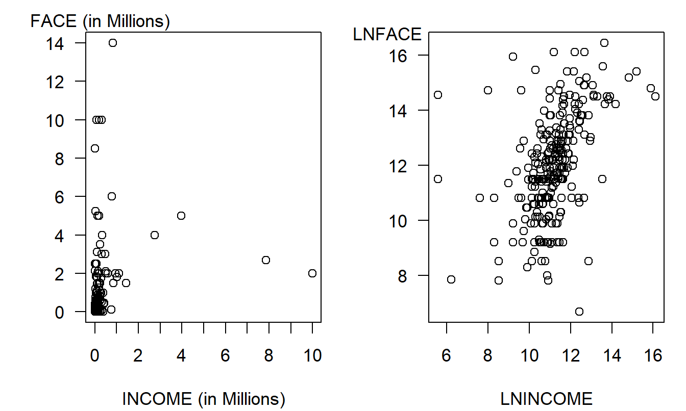
Figure 3.1: Income versus Face Amount of Term Life Insurance. The left-panel is a plot of face versus income, showing a highly nonlinear pattern. In the right-hand panel, face versus income is in natural logarithmic units, suggesting a linear (although variable) pattern.
R Code to Produce Table 3.1 and Figure 3.1
The Term Life data are multivariate in the sense that several measurements are taken on each household. It is difficult to produce a graph of observations in three or more dimensions on a two-dimensional platform, such as a piece of paper, that is not confusing, misleading, or both. To summarize graphically multivariate data in regression applications, consider using a scatterplot matrix such as in Figure 3.2. Each square of this figure represents a simple plot of one variable versus another. For each square, the row variable gives the units of the vertical axis and the column variable gives the units of the horizontal axis. The matrix is sometimes called a half scatterplot matrix because only the lower left-hand elements are presented.
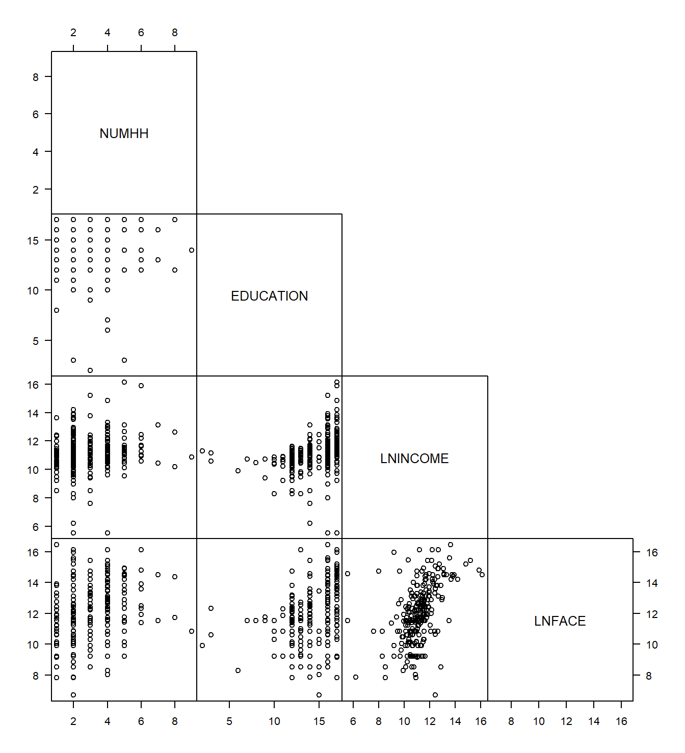
Figure 3.2: Scatterplot matrix of four variables. Each square is a scatter plot.
The scatterplot matrix can be numerically summarized using a correlation matrix. Each correlation in Table 3.2 corresponds to a square of the scatterplot matrix in Figure 3.2. Analysts often present tables of correlations because they are easy to interpret. However, remember that a correlation coefficient merely measures the extent of linear relationships. Thus, a table of correlations provides a sense of linear relationships but may miss a nonlinear relationship that can be revealed in a scatterplot matrix.
| NUMHH | EDUCATION | LNINCOME | |
|---|---|---|---|
| EDUCATION | -0.064 | ||
| LNINCOME | 0.179 | 0.343 | |
| LNFACE | 0.288 | 0.383 | 0.482 |
The scatterplot matrix and corresponding correlation matrix are useful devices for summarizing multivariate data. They are easy to produce and to interpret. Still, each device captures only relationships between pairs of variables and cannot quantify relationships among several variables.
R Code to Produce Table 3.2 and Figure 3.2
Method of Least Squares
Consider the question: “Can knowledge of education, household size, and income help us understand the demand for insurance?” The correlations in Table 3.2 and the graphs in Figures 3.1 and 3.2 suggest that each variable, EDUCATION, NUMHH, and LNINCOME, may be a useful explanatory variable of LNFACE when taken individually. It seems reasonable to investigate the joint effect of these variables on a response.
The geometric concept of a plane is used to explore the linear relationship between a response and several explanatory variables. Recall that a plane extends the concept of a line to more than two dimensions. A plane may be defined through an algebraic equation such as
\[ y = b_0 + b_1 x_1 + \ldots + b_k x_k. \]
This equation defines a plane in \(k+1\) dimensions. Figure 3.3 shows a plane in three dimensions. For this figure, there is one response variable, LNFACE, and two explanatory variables, EDUCATION and LNINCOME (NUMHH is held fixed). It is difficult to graph more than three dimensions in a meaningful way.
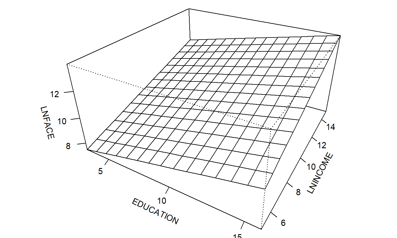
Figure 3.3: An example of a three-dimensional plane
We need a way to determine a plane based on the data. The difficulty is that in most regression analysis applications, the number of observations, \(n\), far exceeds the number of observations required to fit a plane, \(k+1\). Thus, it is generally not possible to find a single plane that passes through all \(n\) observations. As in Chapter 2, we use the method of least squares to determine a plane from the data.
The method of least squares is based on determining the values of \(b_0^{\ast},b_1^{\ast},\ldots,b_k^{\ast}\) that minimize the quantity
\[\begin{equation} SS(b_0^{\ast},b_1^{\ast},\ldots,b_k^{\ast})=\sum_{i=1}^{n}\left( y_i-\left( b_0^{\ast}+b_1^{\ast}x_{i1}+\ldots+b_k^{\ast}x_{ik}\right) \right) ^2. \tag{3.1} \end{equation}\]
We drop the asterisk, or star, notation and use \(b_0, b_1, \ldots, b_k\) to denote the best values, known as the least squares estimates. With the least squares estimates, define the least squares, or fitted, regression plane as
\[ \widehat{y} = b_0 + b_1 x_1 + \ldots + b_k x_k. \]
The least squares estimates are determined by minimizing \(SS(b_0^{\ast},b_1^{\ast},\ldots,b_k^{\ast})\). It is difficult to write down the resulting least squares estimators using a simple formula unless one resorts to matrix notation. Because of their importance in applied statistical models, an explicit formula for the estimators is provided below. However, these formulas have been programmed into a wide variety of statistical and spreadsheet software packages. The availability of these packages allows data analysts to concentrate on the ideas of the estimation procedure instead of focusing on the details of the calculation procedures.
As an example, a regression plane was fit to the Term Life data where three explanatory variables, \(x_1\) for EDUCATION, \(x_2\) for NUMHH, and \(x_3\) for LNINCOME, were used. The resulting fitted regression plane is
\[\begin{equation} \widehat{y} = 2.584 + 0.206 x_1 + 0.306 x_2 + 0.494 x_3. \tag{3.2} \end{equation}\]
Video: Summary
Matrix Notation
Assume that the data are of the form \((x_{i0}, x_{i1}, \ldots, x_{ik}, y_i)\), where \(i = 1, \ldots, n\). Here, the variable \(x_{i0}\) is associated with the “intercept” term. In most applications, we assume that \(x_{i0}\) is identically equal to 1 and thus need not be explicitly represented. However, there are important applications where this is not the case, and thus, to express the model in general notation, it is included here. The data are represented in matrix notation using:
\[ \mathbf{y} = \begin{pmatrix} y_1 \\ y_2 \\ \vdots \\ y_n \end{pmatrix} ~~\text{and}~~ \mathbf{X} = \begin{pmatrix} x_{10} & x_{11} & \cdots & x_{1k} \\ x_{20} & x_{21} & \cdots & x_{2k} \\ \vdots & \vdots & \ddots & \vdots \\ x_{n0} & x_{n1} & \cdots & x_{nk} \end{pmatrix}. \]
Here, \(\mathbf{y}\) is the \(n \times 1\) vector of responses and \(\mathbf{X}\) is the \(n \times (k+1)\) matrix of explanatory variables. We use the matrix algebra convention that lower and upper case bold letters represent vectors and matrices, respectively. (If you need to brush up on matrices, review Section 2.11.)
Example: Term Life Insurance - Continued. Recall that \(y\) represents the logarithmic face, \(x_1\) for years of education, \(x_2\) for the number of household members, and \(x_3\) for logarithmic income. Thus, there are \(k = 3\) explanatory variables and \(n = 275\) households. The vector of responses and the matrix of explanatory variables are:
\[ \mathbf{y} = \begin{pmatrix} y_1 \\ y_2 \\ \vdots \\ y_{275} \end{pmatrix} = \begin{pmatrix} 9.904 \\ 11.775 \\ \vdots \\ 9.210 \end{pmatrix} ~~\text{and}~~ \\ \mathbf{X} = \begin{pmatrix} 1 & x_{11} & x_{12} & x_{13} \\ 1 & x_{21} & x_{22} & x_{23} \\ \vdots & \vdots & \vdots & \vdots \\ 1 & x_{275,1} & x_{275,2} & x_{275,3} \end{pmatrix} = \begin{pmatrix} 1 & 16 & 3 & 10.669 \\ 1 & 9 & 3 & 9.393 \\ \vdots & \vdots & \vdots & \vdots \\ 1 & 12 & 1 & 10.545 \end{pmatrix}. \]
For example, for the first observation in the data set, the dependent variable is \(y_1 = 9.904\) (corresponding to \(\exp(9.904) = \$20,000\)), for a survey respondent with 16 years of education living in a household with 3 people and a logarithmic income of 10.669 (\(\exp(10.669) = \$43,000\)).
Under the least squares estimation principle, our goal is to choose the coefficients \(b_0^{\ast}, b_1^{\ast}, \ldots, b_k^{\ast}\) to minimize the sum of squares function \(SS(b_0^{\ast}, b_1^{\ast}, \ldots, b_k^{\ast})\). Using calculus, we return to the equation for the sum of squares, take partial derivatives with respect to each coefficient, and set these quantities equal to zero:
\[ \begin{array}{ll} \frac{\partial }{\partial b_j^{\ast}}SS(b_0^{\ast}, b_1^{\ast}, \ldots, b_k^{\ast}) &= \sum_{i=1}^{n}\left( -2x_{ij}\right) \left( y_i-\left( b_0^{\ast}+b_1^{\ast}x_{i1}+\ldots+b_k^{\ast}x_{ik}\right) \right) \\ &= 0, ~~~ \text{for} ~ j=0,1,\ldots,k. \end{array} \]
This is a system of \(k+1\) equations and \(k+1\) unknowns that can be readily solved using matrix notation, as follows.
We may express the vector of parameters to be minimized as \(\mathbf{b}^{\ast}=(b_0^{\ast}, b_1^{\ast}, \ldots, b_k^{\ast})^{\prime}\). Using this, the sum of squares can be written as \(SS(\mathbf{b}^{\ast}) = (\mathbf{y-Xb}^{\ast})^{\prime}(\mathbf{y-Xb}^{\ast})\). Thus, in matrix form, the solution to the minimization problem can be expressed as \(\frac{\partial}{\partial \mathbf{b}^{\ast}} SS(\mathbf{b}^{\ast}) = \mathbf{0}\). This solution satisfies the normal equations:
\[\begin{equation} \mathbf{X^{\prime}Xb} = \mathbf{X}^{\prime}\mathbf{y}. \tag{3.3} \end{equation}\]
Here, the asterisk notation (*) has been dropped to denote the fact that \(\mathbf{b} = (b_0, b_1, \ldots, b_k)^{\prime}\) represents the best vector of values in the sense of minimizing \(SS(\mathbf{b}^{\ast})\) over all choices of \(\mathbf{b}^{\ast}\).
The least squares estimator \(\mathbf{b}\) need not be unique. However, assuming that the explanatory variables are not linear combinations of one another, we have that \(\mathbf{X^{\prime}X}\) is invertible. In this case, we can write the unique solution as:
\[\begin{equation} \mathbf{b} = \left( \mathbf{X^{\prime}X} \right)^{-1} \mathbf{X}^{\prime} \mathbf{y}. \tag{3.4} \end{equation}\]
To illustrate, for the Term Life example, equation (3.4) yields:
\[ \mathbf{b} = \begin{pmatrix} b_0 \\ b_1 \\ b_2 \\ b_3 \\ \end{pmatrix} = \begin{pmatrix} 2.584 \\ 0.206 \\ 0.306 \\ 0.494 \\ \end{pmatrix}. \]
Video: Summary
3.2 Linear Regression Model and Properties of Estimators
In the previous section, we learned how to use the method of least squares to fit a regression plane with a data set. This section describes the assumptions underpinning the regression model and some of the resulting properties of the regression coefficient estimators. With the model and the fitted data, we will be able to draw inferences about the sample data set to a larger population. Moreover, we will later use these regression model assumptions to help us improve the model specification in Chapter 5.
3.2.1 Regression Function
Most of the assumptions of the multiple linear regression model will carry over directly from the basic linear regression model assumptions introduced in Section 2.2. The primary difference is that we now summarize the relationship between the response and the explanatory variables through the regression function:
\[\begin{equation} \mathrm{E~}y = \beta_0 x_0 + \beta_1 x_1 + \ldots + \beta_k x_k, \tag{3.5} \end{equation}\]
which is linear in the parameters \(\beta_0,\ldots,\beta_k\). Henceforth, we will use \(x_0 = 1\) for the variable associated with the parameter \(\beta_0\); this is the default in most statistical packages, and most applications of regression include the intercept term \(\beta_0\). The intercept is the expected value of \(y\) when all of the explanatory variables are equal to zero. Although rarely of interest, the term \(\beta_0\) serves to set the height of the fitted regression plane.
In contrast, the other betas are typically important parameters from a regression study. To help interpret them, we initially assume that \(x_j\) varies continuously and is not related to the other explanatory variables. Then, we can interpret \(\beta_j\) as the expected change in \(y\) per unit change in \(x_j\) assuming all other explanatory variables are held fixed. That is, from calculus, you will recognize that \(\beta_j\) can be interpreted as a partial derivative. Specifically, using the equation above, we have that
\[ \beta_j = \frac{\partial }{\partial x_j}\mathrm{E}~y. \]
3.2.2 Regression Coefficient Interpretation
Let us examine the regression coefficient estimates from the Term Life Insurance example and focus initially on the sign of the coefficients. For example, from equation (3.4), the coefficient associated with NUMHH is \(b_2 = 0.306 > 0\). If we consider two households that have the same income and the same level of education, then the larger household (in terms of NUMHH) is expected to demand more term life insurance under the regression model. This is a sensible interpretation; larger households have more dependents for which term life insurance can provide needed financial assets in the event of the untimely death of a breadwinner. The positive coefficient associated with income (\(b_3 = 0.494\)) is also plausible; households with larger incomes have more disposable dollars to purchase insurance. The positive sign associated with EDUCATION (\(b_1 = 0.206)\) is also reasonable; more education suggests that respondents are more aware of their insurance needs, other things being equal.
You will also need to interpret the amount of the regression coefficient. Consider first the EDUCATION coefficient. Using equation (3.4), fitted values of \(\widehat{\mathrm{LNFACE}}\) were calculated by allowing EDUCATION to vary and keeping NUMHH and LNINCOME fixed at the sample averages. The results are:
Effects of Small Changes in Education
| EDUCATION | 14 | 14.1 | 14.2 | 14.3 |
| \(\widehat{\mathit{LNFACE}}\) | 11.883 | 11.904 | 11.924 | 11.945 |
| \(\widehat{\mathit{FACE}}\) | 144,803 | 147,817 | 150,893 | 154,034 |
| \(\widehat{\mathit{FACE}}\) % Change | 2.081 | 2.081 | 2.081 |
As EDUCATION increases, \(\widehat{\mathrm{LNFACE}}\) increases. Further, the amount of \(\widehat{\mathrm{LNFACE}}\) increase is a constant 0.0206. This comes directly from equation (3.4); as EDUCATION increases by 0.1 years, we expect the demand for insurance to increase by 0.0206 logarithmic dollars, holding NUMHH and LNINCOME fixed. This interpretation is correct, but most product development directors are not overly fond of logarithmic dollars. To return to dollars, fitted face values can be calculated through exponentiation as \(\widehat{\mathrm{FACE}} = \exp(\widehat{\mathrm{LNFACE}})\). Moreover, the percentage change can be computed; for example, \(100 \times (147,817/144,803 - 1) \approx 2.08\%\).
This provides another interpretation of the regression coefficient; as EDUCATION increases by 0.1 years, we expect the demand for insurance to increase by 2.08%. This is a simple consequence of calculus using \(\partial \ln y / \partial x = \left(\partial y / \partial x \right) / y\); that is, a small change in the logarithmic value of \(y\) equals a small change in \(y\) as a proportion of \(y\). It is because of this calculus result that we use natural logs instead of common logs in regression analysis. Because this table uses a discrete change in EDUCATION, the 2.08% differs slightly from the continuous result \(0.206 \times (\mathrm{change~in~EDUCATION}) = 2.06\%\). However, this proximity is usually regarded as suitable for interpretation purposes.
Continuing this logic, consider small changes in logarithmic income.
Effects of Small Changes in Logarithmic Income| LNINCOME | 11 | 11.1 | 11.2 | 11.3 |
| INCOME | 59,874 | 66,171 | 73,130 | 80,822 |
| INCOME % Change | 10.52 | 10.52 | 10.52 | |
| \(\widehat{\mathit{LNFACE}}\) | 11.957 | 12.006 | 12.055 | 12.105 |
| \(\widehat{\mathit{FACE}}\) | 155,831 | 163,722 | 172,013 | 180,724 |
| \(\widehat{\mathit{FACE}}\) % Change | 5.06 | 5.06 | 5.06 | |
| \(\widehat{\mathit{FACE}}\) % Change / INCOME % Change | 0.482 | 0.482 | 0.482 |
We can use the same logic to interpret the LNINCOME coefficient in equation (3.4). As logarithmic income increases by 0.1 units, we expect the demand for insurance to increase by 5.06%. This takes care of logarithmic units in the \(y\) but not the \(x\). We can use the same logic to say that as logarithmic income increases by 0.1 units, INCOME increases by 10.52%. Thus, a 10.52% change in INCOME corresponds to a 5.06% change in FACE. Summarizing, we say that, holding NUMHH and EDUCATION fixed, we expect that a 1% increase in INCOME is associated with a 0.482% increase in \(\widehat{\mathrm{FACE}}\) (as before, this is close to the parameter estimate \(b_3 = 0.494\)). The coefficient associated with income is known as an elasticity in economics. In economics, elasticity is the ratio of the percent change in one variable to the percent change in another variable. Mathematically, we summarize this as:
\[ \frac{\partial \ln y}{\partial \ln x} = \left(\frac{\partial y}{y}\right)/\left(\frac{\partial x}{x}\right). \]
Video: Summary
3.2.3 Model Assumptions
As in Section 2.2 for a single explanatory variable, there are two sets of assumptions that one can use for multiple linear regression. They are equivalent sets, each having comparative advantages as we proceed in our study of regression. The “observables” representation focuses on variables of interest \((x_{i1}, \ldots, x_{ik}, y_i)\). The “error representation” provides a springboard for motivating our goodness of fit measures and study of residual analysis. However, the latter set of assumptions focuses on the additive errors case and obscures the sampling basis of the model.
\[ \textbf{Multiple Linear Regression Model Sampling Assumptions} \\ \small{ \begin{array}{ll} \text{Observables Representation} & \text{Error Representation} \\ \hline F1.~ \mathrm{E}~y_i=\beta_0+\beta_1 x_{i1}+\ldots+\beta_k x_{ik}. & E1.~ y_i=\beta_0+\beta_1 x_{i1}+\ldots+\beta_k x_{ik}+\varepsilon_i. \\ F2.~ \{x_{i1},\ldots ,x_{ik}\} & E2.~ \{x_{i1},\ldots ,x_{ik}\} \\ \ \ \ \ \ \ \ \ \text{are non-stochastic variables.} & \ \ \ \ \ \ \ \ \text{are non-stochastic variables.} \\ F3.~ \mathrm{Var}~y_i=\sigma^2. & E3.~ \mathrm{E}~\varepsilon_i=0 \text{ and } \mathrm{Var}~\varepsilon_i=\sigma^2. \\ F4.~ \{y_i\} \text{ are independent random variables.} & E4.~ \{\varepsilon_i\} \text{ are independent random variables.} \\ F5.~ \{y_i\} \text{ are normally distributed.} & E5.~ \{\varepsilon_i\} \text{ are normally distributed.} \\ \hline \end{array} } \]
To further motivate Assumptions F2 and F4, we will usually assume that our data have been realized as the result of a stratified sampling scheme, where each unique value of \(\{x_{i1}, \ldots, x_{ik}\}\) is treated as a stratum. That is, for each value of \(\{x_{i1}, \ldots, x_{ik}\}\), we draw a random sample of responses from a population. Thus, responses within each stratum are independent from one another, as are responses from different strata. Chapter 6 will discuss this sampling basis in further detail.
3.2.4 Properties of Regression Coefficient Estimators
Section 3.1 described the least squares method for estimating regression coefficients. With the regression model assumptions, we can establish some basic properties of these estimators. To do this, from Section 2.11.4 we have that the expectation of a vector is the vector of expectations, so that
\[ \mathrm{E}~\mathbf{y} = \left( \begin{array}{l} \mathrm{E}~y_1 \\ \mathrm{E}~y_2 \\ \vdots \\ \mathrm{E}~y_n \end{array} \right) . \]
Further, basic matrix multiplication shows that
\[ \small{ \mathbf{X} \boldsymbol \beta = \left( \begin{array}{cccc} 1 & x_{11} & \cdots & x_{1k} \\ 1 & x_{21} & \cdots & x_{2k} \\ \vdots & \vdots & \ddots & \vdots \\ 1 & x_{n1} & \cdots & x_{nk} \end{array} \right) \left( \begin{array}{c} \beta_0 \\ \beta_1 \\ \vdots \\ \beta_k \end{array} \right) = \left( \begin{array}{c} \beta_0 + \beta_1 x_{11} + \cdots + \beta_k x_{1k} \\ \beta_0 + \beta_1 x_{21} + \cdots + \beta_k x_{2k} \\ \vdots \\ \beta_0 + \beta_1 x_{n1} + \cdots + \beta_k x_{nk} \end{array} \right) . } \]
Because the \(i\)th row of assumption F1 is \(\mathrm{E}~y_i = \beta_0 + \beta_1 x_{i1} + \cdots + \beta_k x_{ik}\), we may re-write this assumption in matrix formulation as \(\mathrm{E}~\mathbf{y} = \mathbf{X} \boldsymbol \beta\). We are now in a position to state the first important property of least squares regression estimators.
Property 1. Consider a regression model and let Assumptions F1-F4 hold. Then, the estimator \(\mathbf{b}\) defined in equation (3.4) is an unbiased estimator of the parameter vector \(\boldsymbol \beta\).
To establish Property 1, we have that
\[ \mathrm{E}~\mathbf{b} = \mathrm{E}~\left((\mathbf{X^{\prime}X)}^{-1}\mathbf{X}^{\prime}\mathbf{y}\right) = (\mathbf{X^{\prime}X)}^{-1}\mathbf{X}^{\prime}\mathrm{E}~\mathbf{y} = (\mathbf{X^{\prime}X)}^{-1} \mathbf{X}^{\prime} \left( \mathbf{X} \boldsymbol \beta \right) = \boldsymbol \beta, \]
using matrix multiplication rules. This chapter assumes that \(\mathbf{X^{\prime}X}\) is invertible. One can also show that the least squares estimator need only be a solution of the normal equations for unbiasedness (not requiring that \(\mathbf{X^{\prime}X}\) be invertible, see Section 4.7.3). Thus, \(\mathbf{b}\) is said to be an unbiased estimator of \(\boldsymbol \beta\). In particular, \(\mathrm{E}~b_j = \beta_j\) for \(j = 0,1,\ldots,k\).
Because independence implies zero covariance, from Assumption F4 we have that \(\mathrm{Cov}(y_i,y_j) = 0\) for \(i \neq j\). From this, Assumption F3 and the definition of the variance of a vector, we have that
\[ \small{ \mathrm{Var~}\mathbf{y} = \left( \begin{array}{cccc} \mathrm{Var~}y_1 & \mathrm{Cov}(y_1,y_2) & \cdots & \mathrm{Cov}(y_1,y_n) \\ \mathrm{Cov}(y_2,y_1) & \mathrm{Var~}y_2 & \cdots & \mathrm{Cov}(y_2,y_n) \\ \vdots & \vdots & \ddots & \vdots \\ \mathrm{Cov}(y_n,y_1) & \mathrm{Cov}(y_n,y_2) & \cdots & \mathrm{Var~}y_n \end{array} \right) = \left( \begin{array}{cccc} \sigma^2 & 0 & \cdots & 0 \\ 0 & \sigma^2 & \cdots & 0 \\ \vdots & \vdots & \ddots & \vdots \\ 0 & 0 & \cdots & \sigma^2 \end{array} \right) = \sigma^2 \mathbf{I}, } \]
where \(\mathbf{I}\) is an \(n \times n\) identity matrix. We are now in a position to state the second important property of least squares regression estimators.
Property 2. Consider a regression model and let Assumptions F1-F4 hold. Then, the estimator \(\mathbf{b}\) defined in equation (3.4) has variance \(\mathrm{Var~}\mathbf{b} = \sigma^2(\mathbf{X^{\prime}X)}^{-1}\).
To establish Property 2, we have that
\[ \mathrm{Var~}\mathbf{b} = \mathrm{Var}\left((\mathbf{X^{\prime}X)}^{-1} \mathbf{X}^{\prime}\mathbf{y}\right) = \left[ (\mathbf{X^{\prime}X)}^{-1} \mathbf{X}^{\prime}\right] \mathrm{Var}\left( \mathbf{y}\right) \left[\mathbf{X}(\mathbf{X^{\prime}X)}^{-1}\right] \\ = \left[ (\mathbf{X^{\prime}X)}^{-1}\mathbf{X}^{\prime}\right] \sigma^2 \mathbf{I}\left[\mathbf{X}(\mathbf{X^{\prime}X)}^{-1}\right] = \sigma^2(\mathbf{X^{\prime}X)}^{-1}, \]
as required. This important property will allow us to measure the precision of the estimator \(\mathbf{b}\) when we discuss statistical inference. Specifically, by the definition of the variance of a vector (see Section 2.11.4),
\[\begin{equation} \mathrm{Var~}\mathbf{b}= \begin{pmatrix} \mathrm{Var~}b_0 & \mathrm{Cov}(b_0,b_1) & \cdots & \mathrm{Cov}(b_0,b_k) \\ \mathrm{Cov}(b_1,b_0) & \mathrm{Var~}b_1 & \cdots & \mathrm{Cov}(b_1,b_k) \\ \vdots & \vdots & \ddots & \vdots \\ \mathrm{Cov}(b_k,b_0) & \mathrm{Cov}(b_k,b_1) & \cdots & \mathrm{Var~}b_k \end{pmatrix} = \sigma^2 (\mathbf{X^{\prime}X)}^{-1}. \tag{3.6} \end{equation}\]
Thus, for example, \(\mathrm{Var~}b_j\) is \(\sigma^2\) times the \((j+1)\)st diagonal entry of \((\mathbf{X^{\prime}X)}^{-1}\). As another example, \(\mathrm{Cov}(b_0,b_j)\) is \(\sigma^2\) times the element in the first row and \((j+1)\)st column of \((\mathbf{X^{\prime}X)}^{-1}\).
Although alternative methods are available that are preferable for specific applications, the least squares estimators have proven to be effective for many routine data analyses. One desirable characteristic of least squares regression estimators is summarized in the following well-known result.
Gauss-Markov Theorem: Consider the regression model and let Assumptions F1-F4 hold. Then, within the class of estimators that are linear functions of the responses, the least squares estimator \(\mathbf{b}\) defined in equation (3.4) is the minimum variance unbiased estimator of the parameter vector \(\boldsymbol{\beta}\).
The Gauss-Markov theorem states that the least squares estimator is the most precise in the sense that it has the smallest variance.
We have already seen in Property 1 that the least squares estimators are unbiased. The Gauss-Markov theorem states that the least squares estimator is the most precise in the sense that it has the smallest variance. (In a matrix context, “minimum variance” means that if \(\mathbf{b}^{\ast}\) is any other estimator, then the difference of the variance matrices, \(\mathrm{Var~} \mathbf{b}^{\ast} - \mathrm{Var~}\mathbf{b}\), is nonnegative definite.)
An additional important property concerns the distribution of the least squares regression estimators.
Property 3: Consider a regression model and let Assumptions F1-F5 hold. Then, the least squares estimator \(\mathbf{b}\) defined in equation (3.4) is normally distributed.
To establish Property 3, we define the weight vectors, \(\mathbf{w}_i = (\mathbf{X^{\prime}X)}^{-1}(1, x_{i1}, \ldots, x_{ik})^{\prime}\). With this notation, we note that
\[ \mathbf{b} = (\mathbf{X^{\prime}X)}^{-1}\mathbf{X}^{\prime}\mathbf{y} = \sum_{i=1}^{n} \mathbf{w}_i y_i, \]
so that \(\mathbf{b}\) is a linear combination of responses. With Assumption F5, the responses are normally distributed. Because linear combinations of normally distributed random variables are normally distributed, we have the conclusion of Property 3. This result underpins much of the statistical inference that will be presented in Sections 3.4 and 4.2.
Video: Summary
3.3 Estimation and Goodness of Fit
Residual Standard Deviation
Additional properties of the regression coefficient estimators will be discussed when we focus on statistical inference. We now continue our estimation discussion by providing an estimator of the other parameter in the linear regression model, \(\sigma^2\).
Our estimator for \(\sigma^2\) can be developed using the principle of replacing theoretical expectations by sample averages. Examining \(\sigma^2 = \mathrm{E}\left( y-\mathrm{E~}y\right)^2\), replacing the outer expectation by a sample average suggests using the estimator \(n^{-1}\sum_{i=1}^{n}(y_i-\mathrm{E~}y_i)^2\). Because we do not observe \(\mathrm{E}~y_i = \beta_0 + \beta_1 x_{i1} + \cdots + \beta_k x_{ik}\), we use in its place the corresponding observed quantity \(b_0 + b_1 x_{i1} + \ldots + b_k x_{ik} = \widehat{y}_i\). This leads to the following.
Definition. An estimator of \(\sigma^2\), the mean square error (MSE), is defined as
\[\begin{equation} s^2 = \frac{1}{n-(k+1)}\sum_{i=1}^{n}\left( y_i - \widehat{y}_i \right)^2. \tag{3.7} \end{equation}\]
The positive square root, \(s = \sqrt{s^2}\), is called the residual standard deviation.
This expression generalizes the definition in equation (2.3), which is valid for \(k=1\). It turns out, by using \(n-(k+1)\) instead of \(n\) in the denominator of equation (3.7), that \(s^2\) is an unbiased estimator of \(\sigma^2\). Essentially, by using \(\widehat{y}_i\) instead of \(\mathrm{E~}y_i\) in the definition, we have introduced some small dependencies among the deviations from the responses \(y_i - \widehat{y}_i\), thus reducing the overall variability. To compensate for this lower variability, we also reduce the denominator in the definition of \(s^2\).
To provide further intuition on the choice of \(n-(k+1)\) in the definition of \(s^2\), we introduced the concept of residuals in the context of multiple linear regression. From Assumption E1, recall that the random errors can be expressed as \(\varepsilon_i = y_i - (\beta_0 + \beta_1 x_{i1} + \cdots + \beta_k x_{ik})\). Because the parameters \(\beta_0, \ldots, \beta_k\) are not observed, the errors themselves are not observed. Instead, we examine the “estimated errors,” or residuals, defined by \(e_i = y_i - \widehat{y}_i\).
Unlike errors, there exist certain dependencies among the residuals. One dependency is due to the algebraic fact that the average residual is zero. Further, there must be at least \(k+2\) observations for there to be variation in the fit of the plane. If we have only \(k+1\) observations, we could fit a plane to the data perfectly, resulting in no variation in the fit. For example, if \(k=1\), because two observations determine a line, then at least three observations are required to observe any deviation from the line. Because of these dependencies, we have only \(n-(k+1)\) free, or unrestricted, residuals to estimate the variability about the regression plane.
The positive square root of \(s^2\) is our estimator of \(\sigma\). Using residuals, it can be expressed as
\[\begin{equation} s = \sqrt{\frac{1}{n-(k+1)}\sum_{i=1}^{n}e_i^2}. \tag{3.8} \end{equation}\]
Because it is based on residuals, we refer to \(s\) as the residual standard deviation. The quantity \(s\) is a measure of our “typical error.” For this reason, \(s\) is also called the standard error of the estimate.
The Coefficient of Determination: \(R^2\)
To summarize the goodness of fit of the model, as in Chapter 2 we partition the variability into pieces that are “explained” and “unexplained” by the regression fit. Algebraically, the calculations for regression using many variables are similar to the case of using only one variable. Unfortunately, when dealing with many variables, we do lose the easy graphical interpretation such as in Figure 2.4.
Begin with the total sum of squared deviations, \(Total~SS = \sum_{i=1}^{n}\left( y_i - \overline{y} \right)^2\), as our measure of the total variation in the data set. As in equation (2.1), we may then interpret the equation
\[ \small{ \begin{array}{ccccc} \underbrace{y_i - \overline{y}} & = & \underbrace{y_i - \widehat{y}_i} & + & \underbrace{\widehat{y}_i - \overline{y}} \\ \text{total} & = & \text{unexplained} & + & \text{explained} \\ \text{deviation} & & \text{deviation} & & \text{deviation} \end{array} } \]
as the “deviation without knowledge of the explanatory variables equals the deviation not explained by the explanatory variables plus deviation explained by the explanatory variables.” Squaring each side and summing over all observations yields
\[ Total~SS = Error~SS + Regression~SS \]
where \(Error~SS = \sum_{i=1}^{n}\left( y_i - \widehat{y}_i \right)^2\) and \(Regression~SS = \sum_{i=1}^{n}\left( \widehat{y}_i - \overline{y} \right)^2\). As in Section 2.3 for the one explanatory variable case, the sum of the cross-product terms turns out to be zero.
A statistic that summarizes this relationship is the coefficient of determination,
\[ R^2 = \frac{Regression~SS}{Total~SS}. \]
We interpret \(R^2\) to be the proportion of variability explained by the regression function.
If the model is a desirable one for the data, one would expect a strong relationship between the observed responses and those “expected” under the model, the fitted values. An interesting algebraic fact is the following. If one squares the correlation coefficient between the responses and the fitted values, we get the coefficient of determination, that is,
\[ R^2 = \left[ r \left(y, \widehat{y} \right) \right]^2. \]
As a result, \(R\), the positive square root of \(R^2\), is called the multiple correlation coefficient. It can be interpreted as the correlation between the response and the best linear combination of the explanatory variables, the fitted values. (This relationship is developed using matrix algebra in the technical supplement Section 5.10.1.)
The variability decomposition is also summarized using the analysis of variance, or ANOVA, table, as follows.
\[ \small{ \begin{array}{l|lcl} \hline \text{Source} & \text{Sum of Squares} & df & \text{Mean Square} \\ \hline \text{Regression} & Regression~SS & k & Regression~MS \\ \text{Error} & Error~SS & n - (k + 1) & MSE \\ \text{Total} & Total~SS & n - 1 & \\ \hline \end{array} } \]
The mean square column figures are defined to be the sum of squares figures divided by their respective degrees of freedom. The error degrees of freedom denotes the number of unrestricted residuals. It is this number that we use in our definition of the “average,” or mean, square error. That is, we define
\[ MSE = Error~MS = \frac{Error~SS}{n - (k + 1)} = s^2. \]
Similarly, the regression degrees of freedom is the number of explanatory variables. This yields
\[ Regression~MS = \frac{Regression~SS}{k}. \]
When discussing the coefficient of determination, it can be established that whenever an explanatory variable is added to the model, \(R^2\) never decreases. This is true whether or not the additional variable is useful. We would like a measure of fit that decreases when useless variables are entered into the model as explanatory variables. To circumvent this anomaly, a widely used statistic is the coefficient of determination adjusted for degrees of freedom, defined by
\[\begin{equation} R_{a}^2 = 1 - \frac{(Error~SS) / [n - (k + 1)]}{(Total~SS) / (n - 1)} = 1 - \frac{s^2}{s_{y}^2}. \tag{3.9} \end{equation}\]
To interpret this statistic, note that \(s_y^2\) does not depend on the model nor the model variables. Thus, \(s^2\) and \(R_a^2\) are equivalent measures of model fit. As the model fit improves, then \(R_{a}^2\) becomes larger and \(s^2\) becomes smaller, and vice versa. Put another way, choosing a model with the smallest \(s^2\) is equivalent to choosing a model with the largest \(R_a^2\).
Example: Term Life Insurance - Continued. To illustrate, Table 3.3 displays the summary statistics for the regression of LNFACE on EDUCATION, NUMHH, and LNINCOME. From the degrees of freedom column, we remind ourselves that there are three explanatory variables and 275 observations. As measures of model fit, the coefficient of determination is \(R^2 = 34.3\%\) (=\(328.47 / 958.90\)) and the residual standard deviation is \(s = 1.525\) (=\(\sqrt{2.326}\)). If we were to attempt to estimate the logarithmic face amount without knowledge of the explanatory variables EDUCATION, NUMHH, and LNINCOME, then the size of the typical error would be \(s_y = 1.871\) (=\(\sqrt{958.90 / 274}\)). Thus, by taking advantage of our knowledge of the explanatory variables, we have been able to reduce the size of the typical error. The measure of model fit that compares these two estimates of variability is the adjusted coefficient of determination, \(R_a^2 = 1 - 2.326 / 1.871^2 = 33.6\%\).
| Sum of Squares | \(df\) | Mean Square | |
|---|---|---|---|
| Regression | 328.47 | 3 | 109.49 |
| Error | 630.43 | 271 | 2.326 |
| Total | 958.9 | 274 |
Example: Why do Females Live Longer than Males? In an article with this title, Lemaire (2002) examined what he called the “female advantage,” the difference in life expectancy between females and males. Life expectancies are of interest because they are widely used measures of a nation’s health. Lemaire examined data from \(n = 169\) countries and found that the average female advantage was 4.51 years worldwide. He sought to explain this difference based on 45 behavioral measures, variables that capture a nation’s degree of economic modernization, social/cultural/religious mores, geographic position, and quality of health care available.
After a detailed analysis, Lemaire reports coefficients from a regression model that appear in Table 3.4. This regression model explains \(R^2 = 61\%\) of the variability. It is a parsimonious model consisting of only \(k = 4\) of the original 45 variables.
Table 3.4. Regression Coefficients from a Model of Female Advantage
\[ \small{ \begin{array}{l|rr} \hline \text{Variable} & \text{Coefficient} & t\text{-statistic} \\ \hline \text{Intercept} & 9.904 & 12.928 \\ \text{Logarithmic Number of Persons per Physician} & -0.473 & -3.212 \\ \text{Fertility} & -0.444 & -3.477 \\ \text{Percentage of Hindus and Buddhists} & -0.018 & -3.196 \\ \text{Soviet Union Dummy} & 4.922 & 7.235 \\ \hline \end{array} } \]
Source: Lemaire (2002)
All variables were strongly statistically significant. The number of persons per physician was also correlated with other variables that capture a country’s degree of economic modernization, such as urbanization, number of cars, and the percentage working in agriculture. Fertility, the number of births per woman, was highly correlated with education variables in the study, including female illiteracy and female school enrollment. The percentage of Hindus and Buddhists is a social/cultural/religious variable. The Soviet Union dummy is a geographic variable - it characterizes Eastern European countries that formerly belonged to the Soviet Union. Because of the high degree of collinearity among the 45 candidate variables, other analysts could easily pick an alternative set of variables. Nonetheless, Lemaire’s important point was that this simple model explains roughly 61% of the variability based on only behavioral variables, unrelated to biological sex differences.
Video: Section Summary
3.4 Statistical Inference for a Single Coefficient
3.4.1 The t-Test
In many applications, a single variable is of primary interest, and other variables are included in the regression to control for additional sources of variability. To illustrate, a sales agent might be interested in the effect that income has on the quantity of insurance demanded. In a regression analysis, one could also include other explanatory variables such as an individual’s gender, type of occupation, age, size of the household, education level, and so on. By including these additional explanatory variables, we hope to gain a better understanding of the relationship between income and insurance demand. To reach sensible conclusions, we will need some rules to decide whether a variable is important or not.
We respond to the question “Is \(x_j\) important?” by investigating whether or not the corresponding slope parameter, \(\beta_j\), equals zero. The question is whether \(\beta_j\) is zero can be restated in the hypothesis testing framework as “Is \(H_0:\beta_j=0\) valid?”
We examine the proximity of \(b_j\) to zero in order to determine whether or not \(\beta_j\) is zero. Because the units of \(b_j\) depend on the units of \(y\) and \(x_j\), we need to standardize this quantity. From Property 2 and equation (3.6), we saw that \(\mathrm{Var~}b_j\) is \(\sigma^2\) times the \((j+1)^{st}\) diagonal element of \((\mathbf{X^{\prime}X})^{-1}\). Replacing \(\sigma^2\) by the estimator \(s^2\) and taking square roots, we have the following.
Definition. The standard error of \(b_j\) can be expressed as
\[ se(b_j) = s \sqrt{\text{(j+1)st diagonal element of } (\mathbf{X^{\prime}X})^{-1}}. \]
Recall that a standard error is an estimated standard deviation. To test \(H_0:\beta_j=0\), we examine the \(t\)-ratio, \(t(b_j) = \frac{b_j}{se(b_j)}\). We interpret \(t(b_j)\) to be the number of standard errors that \(b_j\) is away from zero. This is the appropriate quantity because the sampling distribution of \(t(b_j)\) can be shown to be the \(t\)-distribution with \(df=n-(k+1)\) degrees of freedom, under the null hypothesis with the linear regression model assumptions F1-F5. This enables us to construct tests of the null hypothesis such as the following procedure:
Procedure. The t-test for a Regression Coefficient (\(\beta\)).
- The null hypothesis is \(H_0:\beta_j=0\).
- The alternative hypothesis is \(H_{a}:\beta_j \neq 0\).
- Establish a significance level \(\alpha\) (typically but not necessarily 5%).
- Construct the statistic, \(t(b_j) = \frac{b_j}{se(b_j)}\).
- Procedure: Reject the null hypothesis in favor of the alternative if \(|t(b_j)|\) exceeds a \(t\)-value. Here, this \(t\)-value is the \((1-\alpha /2)^{th}\) percentile from the \(t\)-distribution using \(df=n-(k+1)\) degrees of freedom, denoted as \(t_{n-(k+1),1-\alpha /2}\).
In many applications, the sample size will be large enough so that we may approximate the \(t\)-value by the corresponding percentile from the standard normal curve. At the 5% level of significance, this percentile is 1.96. Thus, as a rule of thumb, we can interpret a variable to be important if its \(t\)-ratio exceeds two in absolute value.
Although it is the most common, testing \(H_0:\beta_j=0\) versus \(H_{a}:\beta_j \neq 0\) is just one of many hypothesis tests that can be performed. Table 3.5 outlines alternative decision-making procedures. These procedures are for testing \(H_0:\beta_j = d\). Here, \(d\) is a user-prescribed value that may be equal to zero or any other known value.
Table 3.5. Decision-Making Procedures for Testing \(H_0: \beta_j = d\)
\[ \small{ \begin{array}{cc} \hline \text{Alternative Hypothesis }(H_{a}) & \text{Procedure: Reject } H_0 \text{ in favor of } H_a \text{ if }\\ \hline \beta_j > d & t-\mathrm{ratio}>t_{n-(k+1),1-\alpha } \\ \beta_j < d & t-\mathrm{ratio}<-t_{n-(k+1),1-\alpha } \\ \beta_j\neq d & |t-\mathrm{ratio}\mathit{|}>t_{n-(k+1),1-\alpha/2} \end{array} \\ \begin{array}{ll}\hline \textit{Notes:} &\text{ The significance level is } \alpha. \text{ Here, } t_{n-(k+1),1-\alpha}\text{ is the }(1-\alpha)^{th}\text{ percentile} \\ &~~\text{from the }t-\text{distribution using } df=n-(k+1)\text{ degrees of freedom.} \\ &~~\text{The test statistic is }t-\mathrm{ratio} = (b_j -d)/se(b_j) . \\ \hline \end{array} } \]
Alternatively, one can construct \(p\)-values and compare these to given significant levels. The \(p\)-value allows the report reader to understand the strength of the deviation from the null hypothesis. Table 3.6 summarizes the procedure for calculating \(p\)-values.
Table 3.6. Probability Values for Testing \(H_0:\beta_j =d\)
\[ \small{ \begin{array}{cccc} \hline \text{Alternative} & & & \\ \text{Hypothesis} (H_a ) & \beta_j > d & \beta_j < d & \beta_j \neq d \\ \hline p-value & \Pr(t_{n-(k+1)}>t-ratio) & \Pr(t_{n-(k+1)}<t-ratio) & \Pr(|t_{n-(k+1)}|>|t-ratio|) \\ \end{array} \\ \begin{array}{ll}\hline \textit{Notes:} & \text{ Here, } t_{n-(k+1)} \text{ is a }t\text{-distributed random variable with }df=n-(k+1)\text{ degrees of freedom.} \\ &~~\text{The test statistic is }t-\mathrm{ratio} = (b_j -d)/se(b_j) . \\ \hline \end{array} } \]
Example: Term Life Insurance - Continued. A useful convention when reporting the results of a statistical analysis is to place the standard error of a statistic in parenthesis below that statistic. Thus, for example, in our regression of LNFACE on EDUCATION, NUMHH, and LNINCOME, the estimated regression equation is:
\[ \begin{array}{lccccc} \widehat{LNFACE} = &2.584 ~ + &0.206~ \text{EDUCATION} + &0.306 ~\text{NUMHH} + &0.494 ~\text{LNINCOME}. \\ \text{std error} &(0.846) &(0.039) &(0.063) &(0.078). \end{array} \]
To illustrate the calculation of the standard errors, first note that from Table 3.3 we have that the residual standard deviation is \(s=1.525\). Using a statistical package, we have
\[ \small{ (\mathbf{X^{\prime}X})^{-1} = \begin{pmatrix} 0.307975 & -0.004633 & -0.002131 & -0.020697 \\ -0.004633 & 0.000648 & 0.000143 & -0.000467 \\ -0.002131 & 0.000143 & 0.001724 & -0.000453 \\ -0.020697 & -0.000467 & -0.000453 & 0.002585 \end{pmatrix}. } \]
To illustrate, we can compute \(se(b_3)=s \times \sqrt{0.002585} = 0.078\), as above. Calculation of the standard errors, as well as the corresponding \(t\)-statistics, is part of the standard output from statistical software and need not be computed by users. Our purpose here is to illustrate the ideas underlying the routine calculations.
With this information, we can immediately compute \(t\)-ratios to check whether a coefficient associated with an individual variable is significantly different from zero. For example, the \(t\)-ratio for the LNINCOME variable is \(t(b_3) = \frac{0.494}{0.078} = 6.3\). The interpretation is that \(b_3\) is over four standard errors above zero and thus LNINCOME is an important variable in the model. More formally, we may be interested in testing the null hypothesis that \(H_0:\beta_3 = 0\) versus \(H_0:\beta_3 \neq 0\). At a 5% level of significance, the \(t\)-value is 1.96, because \(df=275-(1+3)=271\). We thus reject the null in favor of the alternative hypothesis, that logarithmic income (LNINCOME) is important in determining the logarithmic face amount.
3.4.2 Confidence Intervals
Confidence intervals for parameters represent another device for describing the strength of the contribution of the \(j\)th explanatory variable. The statistic \(b_j\) is called a point estimate of the parameter \(\beta_j\). To provide a range of reliability, we use the confidence interval:
\[\begin{equation} b_j \pm t_{n-(k+1),1-\alpha /2}~se(b_j). \tag{3.10} \end{equation}\]
Here, the \(t\)-value \(t_{n-(k+1),1-\alpha /2}\) is a percentile from the \(t\)-distribution with \(df=n-(k+1)\) degrees of freedom. We use the same \(t\)-value as in the two-sided hypothesis test. Indeed, there is a duality between the confidence interval and the two-sided hypothesis test. For example, it is not hard to check that if a hypothesized value falls outside the confidence interval, then \(H_0\) will be rejected in favor of \(H_{a}\). Further, knowledge of the \(p\)-value, point estimate, and standard error can be used to determine a confidence interval.
Video: Section Summary
3.4.3 Added Variable Plots
To represent multivariate data graphically, we have seen that a scatterplot matrix is a useful device. However, the major shortcoming of the scatterplot matrix is that it only captures relationships between pairs of variables. When the data can be summarized using a regression model, a graphical device that does not have this shortcoming is an added variable plot. The added variable plot is also called a partial regression plot because, as we will see, it is constructed in terms of residuals from certain regression fits. We will also see that the added variable plot can be summarized in terms of a partial correlation coefficient, thus providing a link between correlation and regression. To introduce these ideas, we work in the context of the following example.
Example: Refrigerator Prices. What characteristics of a refrigerator are important in determining its price (PRICE)? We consider here several characteristics of a refrigerator, including the size of the refrigerator in cubic feet (RSIZE), the size of the freezer compartment in cubic feet (FSIZE), the average amount of money spent per year to operate the refrigerator (ECOST, for “energy cost”), the number of shelves in the refrigerator and freezer doors (SHELVES), and the number of features (FEATURES). The features variable includes shelves for cans, see-through crispers, ice makers, egg racks, and so on.
Both consumers and manufacturers are interested in models of refrigerator prices. Other things equal, consumers generally prefer larger refrigerators with lower energy costs that have more features. Due to forces of supply and demand, we would expect consumers to pay more for these refrigerators. A larger refrigerator with lower energy costs that has more features at a similar price is considered a bargain to the consumer. How much extra would the consumer be willing to pay for this additional space? A model of prices for refrigerators on the market provides some insight into this question.
To this end, we analyze data from \(n=37\) refrigerators. Table 3.7 provides the basic summary statistics for the response variable PRICE and the five explanatory variables. From this table, we see that the average refrigerator price is \(\overline{y} = \$626.40\), with standard deviation \(s_{y} = \$139.80\). Similarly, the average annual amount to operate a refrigerator, or average ECOST, is $70.51.
| Mean | Median | Standard Deviation | Minimum | Maximum | |
|---|---|---|---|---|---|
| ECOST | 70.514 | 68.0 | 9.140 | 60.0 | 94.0 |
| RSIZE | 13.400 | 13.2 | 0.600 | 12.6 | 14.7 |
| FSIZE | 5.184 | 5.1 | 0.938 | 4.1 | 7.4 |
| SHELVES | 2.514 | 2.0 | 1.121 | 1.0 | 5.0 |
| FEATURES | 3.459 | 3.0 | 2.512 | 1.0 | 12.0 |
| PRICE | 626.351 | 590.0 | 139.790 | 460.0 | 1200.0 |
To analyze relationships among pairs of variables, Table 3.8 provides a matrix of correlation coefficients. From the table, we see that there are strong linear relationships between PRICE and each of freezer space (FSIZE) and the number of FEATURES. Surprisingly, there is also a strong positive correlation between PRICE and ECOST. Recall that ECOST is the energy cost; one might expect that higher-priced refrigerators should enjoy lower energy costs.
| ECOST | RSIZE | FSIZE | SHELVES | FEATURES | |
|---|---|---|---|---|---|
| RSIZE | -0.033 | ||||
| FSIZE | 0.855 | -0.235 | |||
| SHELVES | 0.188 | -0.363 | 0.251 | ||
| FEATURES | 0.334 | -0.096 | 0.439 | 0.16 | |
| PRICE | 0.522 | -0.024 | 0.72 | 0.4 | 0.697 |
R Code to Produce Tables 3.7 and 3.8
A regression model was fit to the data. The fitted regression equation appears in Table 3.9, with \(s=60.65\) and \(R^2=83.8\%\).
| Coefficient | Standard Error | \(t\)-Ratio | |
|---|---|---|---|
| Intercept | 798.00 | 271.400 | -2.9 |
| ECOST | -6.96 | 2.275 | -3.1 |
| RSIZE | 76.50 | 19.440 | 3.9 |
| FSIZE | 137.00 | 23.760 | 5.8 |
| SHELVES | 37.90 | 9.886 | 3.8 |
| FEATURES | 23.80 | 4.512 | 5.3 |
From Table 3.9, the explanatory variables seem to be useful predictors of refrigerator prices. Together, these variables account for 83.8% of the variability. For understanding prices, the typical error has dropped from \(s_{y} = \$139.80\) to \(s = \$60.65\). The \(t\)-ratios for each of the explanatory variables exceed two in absolute value, indicating that each variable is important on an individual basis.
What is surprising about the regression fit is the negative coefficient associated with energy cost. Remember, we can interpret \(b_{ECOST} = -6.96\) to mean that, for each dollar increase in ECOST, we expect the PRICE to decrease by $6.96. This negative relationship conforms to our economic intuition. However, it is surprising that the same data set has shown us that there is a positive relationship between PRICE and ECOST. This seeming anomaly is because correlation only measures relationships between pairs of variables although the regression fit can account for several variables simultaneously. To provide more insight into this seeming anomaly, we now introduce the added variable plot.
Producing an Added Variable Plot
The added variable plot provides additional links between the regression methodology and more fundamental tools such as scatter plots and correlations. We work in the context of the Refrigerator Price Example to demonstrate the construction of this plot.
Procedure for producing an added variable plot.
- Run a regression of PRICE on RSIZE, FSIZE, SHELVES, and FEATURES, omitting ECOST. Compute the residuals from this regression, which we label \(e_1\).
- Run a regression of ECOST on RSIZE, FSIZE, SHELVES, and FEATURES. Compute the residuals from this regression, which we label \(e_2\).
- Plot \(e_1\) versus \(e_2\). This is the added variable plot of PRICE versus ECOST, controlling for the effects of the RSIZE, FSIZE, SHELVES, and FEATURES. This plot appears in Figure 3.4.
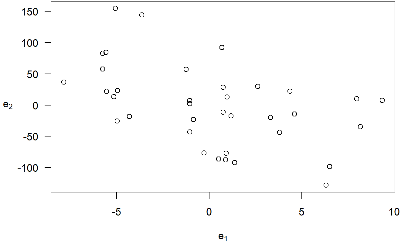
Figure 3.4: An added variable plot. The residuals from the regression of PRICE on the explanatory variables, omitting ECOST, are on the horizontal axis. On the vertical axis are the residuals from the regression fit of ECOST on the other explanatory variables. The correlation coefficient is -0.48.
R Code to Produce Figure 3.4
The error \(\varepsilon\) can be interpreted as the natural variation in a sample. In many situations, this natural variation is small compared to the patterns evident in the nonrandom regression component. Thus, it is useful to think of the error, \(\varepsilon_i = y_i - \left( \beta_0 + \beta_1 x_{i1} + \ldots + \beta_k x_{ik} \right)\), as the response after controlling for the effects of the explanatory variables. In Section 3.3, we saw that a random error can be approximated by a residual, \(e_i = y_i - \left( b_0 + b_1 x_{i1} + \cdots + b_k x_{ik} \right)\). Thus, in the same way, we may think of a residual as the response after “controlling for” the effects of the explanatory variables.
With this in mind, we can interpret the vertical axis of Figure 3.4 as the refrigerator PRICE controlled for effects of RSIZE, FSIZE, SHELVES, and FEATURES. Similarly, we can interpret the horizontal axis as the ECOST controlled for effects of RSIZE, FSIZE, SHELVES, and FEATURES. The plot then provides a graphical representation of the relation between PRICE and ECOST, after controlling for the other explanatory variables. For comparison, a scatter plot of PRICE and ECOST (not shown here) does not control for other explanatory variables. Thus, it is possible that the positive relationship between PRICE and ECOST is not due to a causal relationship but rather one or more additional variables that cause both variables to be large.
For example, from Table 3.8, we see that the freezer size (FSIZE) is positively correlated with both ECOST and PRICE. It certainly seems reasonable that increasing the size of a freezer would cause both the energy cost and the price to increase. Rather, the positive correlation may be due to the fact that large values of FSIZE mean large values of both ECOST and PRICE.
Variables left out of a regression are called omitted variables. This omission could cause a serious problem in a regression model fit; regression coefficients could be not only strongly significant when they should not be, but they may also be of the incorrect sign. Selecting the proper set of variables to be included in the regression model is an important task; it is the subject of Chapters 5 and 6.
3.4.4 Partial Correlation Coefficients
As we saw in Chapter 2, a correlation statistic is a useful quantity for summarizing plots. The correlation for the added variable plot is called a partial correlation coefficient. It is defined to be the correlation between the residuals \(e_1\) and \(e_2\) and is denoted by \(r(y,x_j | x_1, \ldots, x_{j-1}, x_{j+1}, \ldots, x_k)\). Because it summarizes an added variable plot, we may interpret \(r(y,x_j | x_1, \ldots, x_{j-1}, x_{j+1}, \ldots, x_k)\) to be the correlation between \(y\) and \(x_j\), in the presence of the other explanatory variables. To illustrate, the correlation between PRICE and ECOST in the presence of the other explanatory variables is -0.48.
The partial correlation coefficient can also be calculated using
\[\begin{equation} r(y,x_j | x_1, \ldots, x_{j-1}, x_{j+1}, \ldots, x_k) = \frac{t(b_j)}{\sqrt{t(b_j)^2 + n - (k + 1)}}. \tag{3.11} \end{equation}\]
Here, \(t(b_j)\) is the \(t\)-ratio for \(b_j\) from a regression of \(y\) on \(x_1, \ldots, x_k\) (including the variable \(x_j\)). An important aspect of this equation is that it allows us to calculate partial correlation coefficients running only one regression. For example, from Table 3.9, the partial correlation between PRICE and ECOST in the presence of the other explanatory variables is \(\frac{-3.1}{\sqrt{(-3.1)^2 + 37 - (5 + 1)}} \approx -0.48\).
Calculation of partial correlation coefficients is quicker when using the relationship with the \(t\)-ratio, but may fail to detect nonlinear relationships. The information in Table 3.9 allows us to calculate all five partial correlation coefficients in the Refrigerator Price Example after running only one regression. The three-step procedure for producing added variable plots requires ten regressions, two for each of the five explanatory variables. Of course, by producing added variable plots, we can detect nonlinear relationships that are missed by correlation coefficients.
Partial correlation coefficients provide another interpretation for \(t\)-ratios. The equation shows how to calculate a correlation statistic from a \(t\)-ratio, thus providing another link between correlation and regression analysis. Moreover, from the equation we see that the larger the \(t\)-ratio, the larger the partial correlation coefficient. That is, a large \(t\)-ratio means that there is a large correlation between the response and the explanatory variable, controlling for other explanatory variables. This provides a partial response to the question that is regularly asked by consumers of regression analyses, “Which variable is most important?”
Video: Section Summary
3.5 Some Special Explanatory Variables
The linear regression model is the basis of a rich family of models. This section provides several examples to illustrate the richness of this family. These examples demonstrate the use of (i) binary variables, (ii) transformation of explanatory variables, and (iii) interaction terms. This section also serves to underscore the meaning of the adjective linear in the phrase “linear regression”; the regression function is linear in the parameters but may be a highly nonlinear function of the explanatory variables.
3.5.1 Binary Variables
Categorical variables provide a numerical label for measurements of observations that fall in distinct groups, or categories. Because of the grouping, categorical variables are discrete and generally take on a finite number of values. We begin our discussion with a categorical variable that can take on one of only two values, a binary variable. Further discussion of categorical variables is the topic of Chapter 4.
Example: Term Life Insurance - Continued. We now consider the marital status of the survey respondent. In the Survey of Consumer Finances, respondents can select among several options describing their marital status including “married,” “living with a partner,” “divorced,” and so on. Marital status is not measured continuously but rather takes on values that fall into distinct groups. In this chapter, we group survey respondents according to whether or not they are single, defined to include those who are separated, divorced, widowed, never married, and are not married nor living with a partner. Chapter 4 will present a more complete analysis of marital status by including additional categories.
The binary variable SINGLE is defined to be one if the survey respondent is single and 0 otherwise. The variable SINGLE is also known as an indicator variable because it indicates whether or not the respondent is single. Another name for this important type of variable is a dummy variable. We could use 0 and 100, or 20 and 36, or any other distinct values. However, 0 and 1 are convenient for the interpretation of the parameter values, discussed below. To streamline the discussion, we now present a model using only LNINCOME and SINGLE as explanatory variables.
For our sample of \(n = 275\) households, 57 are single and the other 218 are not. To see the relationships among LNFACE, LNINCOME, and SINGLE, Figure 3.5 introduces a letter plot of LNFACE versus LNINCOME, with SINGLE as the code variable. We can see that Figure 3.5 is a scatter plot of LNFACE versus LNINCOME, using 50 randomly selected households from our sample of 275 (for clarity of the graph). However, instead of using the same plotting symbol for each observation, we have coded the symbols so that we can easily understand the behavior of a third variable, SINGLE. In other applications, you may elect to use other plotting symbols such as \(\clubsuit\), \(\heartsuit\), \(\spadesuit\), and so on, or use different colors, to encode additional information. For this application, the letter codes “S” for single and “o” for other were selected because they remind the reader of the nature of the coding scheme. Regardless of the coding scheme, the important point is that a letter plot is a useful device for graphically portraying three or more variables in two dimensions. The main restriction is that the additional information must be categorized, such as with binary variables, to make the coding scheme work.
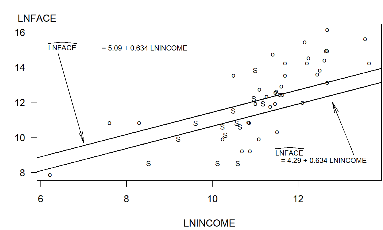
Figure 3.5: Letter plot of LNFACE versus LNINCOME, with the letter code ‘S’ for single and ‘o’ for other. The fitted regression lines have been superimposed. The lower line is for single and the upper line is for other.
Figure 3.5 suggests that LNFACE is lower for those single than others for a given level of income. Thus, we now consider a regression model, LNFACE = β_0 + β_1 LNINCOME + β_2 SINGLE + ϵ. The regression function can be written as:
\[ \text{E } y = \begin{cases} \beta_0 + \beta_1 \text{ LNINCOME} & \text{for other respondents} \\ \beta_0 + \beta_2 + \beta_1 \text{ LNINCOME} & \text{for single respondents} \end{cases} \]
The interpretation of the model coefficients differs from the continuous variable case. For continuous variables such as LNINCOME, we interpret \(\beta_1\) as the expected change in \(y\) per unit change of logarithmic income, holding other variables fixed. For binary variables such as SINGLE, we interpret \(\beta_2\) as the expected increase in \(y\) when going from the base level of SINGLE (=0) to the alternative level. Thus, although we have one model for both marital statuses, we can interpret the model using two regression equations, one for each type of marital status. By writing a separate equation for each marital status, we have been able to simplify a complicated multiple regression equation. Sometimes, you will find it easier to communicate a series of simple relationships compared to a single, complex relationship.
Although the interpretation for binary explanatory variables differs from the continuous, the ordinary least squares estimation method remains valid. To illustrate, the fitted version of the above model is
\[ \small{ \begin{array}{ccccc} \widehat{LNFACE} & = & 5.09 & + 0.634 \text{ LNINCOME} & - 0.800 \text{ SINGLE} .\\ \text{std error} & & (0.89) & ~~(0.078) & ~(0.248) \\ \end{array} } \]
To interpret \(b_2 = -0.800\), we say that we expect the logarithmic face to be smaller by 0.80 for a survey respondent who is single compared to the other category. This assumes that other things, such as income, remain unchanged. For a graphical interpretation, the two fitted regression lines are superimposed in Figure 3.5.
3.5.2 Transforming Explanatory Variables
Regression models have the ability to represent complex, nonlinear relationships between the expected response and the explanatory variables. For example, early regression texts, such as Plackett (1960, Chapter 6), devote an entire chapter of material to polynomial regression,
\[\begin{equation} \text{E } y = \beta_0 + \beta_1 x + \beta_2 x^2 + \ldots + \beta_p x^p. \tag{3.12} \end{equation}\]
Here, the idea is that a \(p\)th order polynomial in \(x\) can be used to approximate general, unknown nonlinear functions of \(x\).
The modern-day treatment of polynomial regression does not require an entire chapter because the model in equation (3.12) can be expressed as a special case of the linear regression model. That is, with the regression function in equation (3.5), \(\text{E } y = \beta_0 + \beta_1 x_1 + \beta_2 x_2 + \ldots + \beta_k x_k\), we can choose \(k = p\) and \(x_1 =x\), \(x_2 = x^2\), \(\ldots\), \(x_p = x^p\). Thus, with these choices of explanatory variables, we can model a highly nonlinear function of \(x\).
We are not restricted to powers of \(x\) in our choice of transformations. For example, the model \(\text{E } y = \beta_0 + \beta_1 \ln x\), provides another way to represent a gently sloping curve in \(x\). This model can be written as a special case of the basic linear regression model using \(x^{\ast} = \ln x\) as the transformed version of \(x\).
Transformations of explanatory variables need not be smooth functions. To illustrate, in some applications, it is useful to categorize a continuous explanatory variable. For example, suppose that \(x\) represents the number of years of education, ranging from 0 to 17. If we are relying on information self-reported by our sample of senior citizens, there may be a substantial amount of error in the measurement of \(x\). We could elect to use a less informative, but more reliable, transform of \(x\) such as \(x^{\ast}\), a binary variable for finishing 13 years of school (finishing high school). Formally, we would code \(x^{\ast} = 1\) if \(x \geq 13\) and \(x^{\ast} = 0\) if \(x < 13\).
Thus, there are several ways that nonlinear functions of the explanatory variables can be used in the regression model. An example of a nonlinear regression model is \(y = \beta_0 + \exp (\beta_1 x) + \varepsilon.\) These typically arise in science applications of regressions where there are fundamental scientific principles guiding the complex model development.
3.5.3 Interaction Terms
We have so far discussed how explanatory variables, say \(x_1\) and \(x_2\), affect the mean response in an additive fashion, that is, \(\mathrm{E}~y = \beta_0 + \beta_1 x_1 + \beta_2 x_2\). Here, we expect \(y\) to increase by \(\beta_1\) per unit increase in \(x_1\), with \(x_2\) held fixed. What if the marginal rate of increase of \(\mathrm{E}~y\) differs for high values of \(x_2\) when compared to low values of \(x_2\)? One way to represent this is to create an interaction variable \(x_3 = x_1 \times x_2\) and consider the model \(\mathrm{E}~y = \beta_0 + \beta_1 x_1 + \beta_2 x_2 + \beta_3 x_3\).
With this model, the change in the expected \(y\) per unit change in \(x_1\) now depends on \(x_2\). Formally, we can assess small changes in the regression function as:
\[ \frac{\partial ~\mathrm{E}~y}{\partial x_1} = \frac{\partial}{\partial x_1} \left(\beta_0 + \beta_1 x_1 + \beta_2 x_2 + \beta_3 x_1 x_2 \right) = \beta_1 + \beta_3 x_2 . \]
In this way, we may allow for more complicated functions of \(x_1\) and \(x_2\). Figure 3.6 illustrates this complex structure. From this figure and the above calculations, we see that the partial changes of \(\mathrm{E}~y\) due to movement of \(x_1\) depend on the value of \(x_2\). In this way, we say that the partial changes due to each variable are not unrelated but rather “move together.”
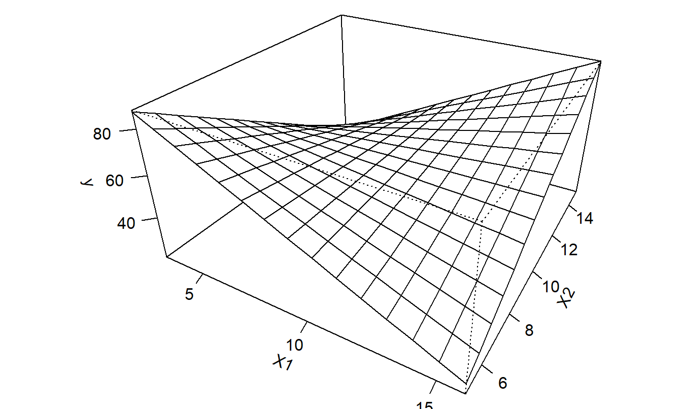
Figure 3.6: Plot of \(\mathrm{E}~y = \beta_0 + \beta_1 x_1 + \beta_2 x_2 + \beta_3 x_1 x_2\) versus \(x_1\) and \(x_2\).
More generally, an interaction term is a variable that is created as a nonlinear function of two or more explanatory variables. These special terms, even though permitting us to explore a rich family of nonlinear functions, can be cast as special cases of the linear regression model. To do this, we simply create the variable of interest and treat this new term as another explanatory variable. Of course, not every variable that we create will be useful. In some instances, the created variable will be so similar to variables already in our model that it will provide us with no new information. Fortunately, we can use \(t\)-tests to check whether the new variable is useful. Further, Chapter 4 will introduce a test to decide whether a group of variables is useful.
The function that we use to create an interaction variable must be more than just a linear combination of other explanatory variables. For example, if we use \(x_3 = x_1 + x_2\), we will not be able to estimate all of the parameters. Chapter 5 will introduce some techniques to help avoid situations when one variable is a linear combination of the others.
To give you some exposure to the wide variety of potential applications of special explanatory variables, we now present a series of short examples.
Example: Term Life Insurance - Continued. How do we interpret the interaction of a binary variable with a continuous variable? To illustrate, consider a Term Life regression model,
\[ \mathrm{LNFACE} = \beta_0 + \beta_1 \mathrm{LNINCOME} + \beta_2 \mathrm{SINGLE} + \beta_3 \mathrm{LNINCOME*SINGLE} + \varepsilon . \]
In this model, we have created a third explanatory variable through the interaction of LNINCOME and SINGLE. The regression function can be written as:
\[ \mathrm{E}~y = \begin{cases} \beta_0 + \beta_1 \mathrm{LNINCOME}, & \text{for other respondents}, \\ \beta_0 + \beta_2 + (\beta_1 + \beta_3) \mathrm{LNINCOME}, & \text{for single respondents}. \end{cases} \]
Thus, through this single model with four parameters, we can create two separate regression lines, one for those single and one for others. Figure 3.7 shows the two fitted regression lines for our data.
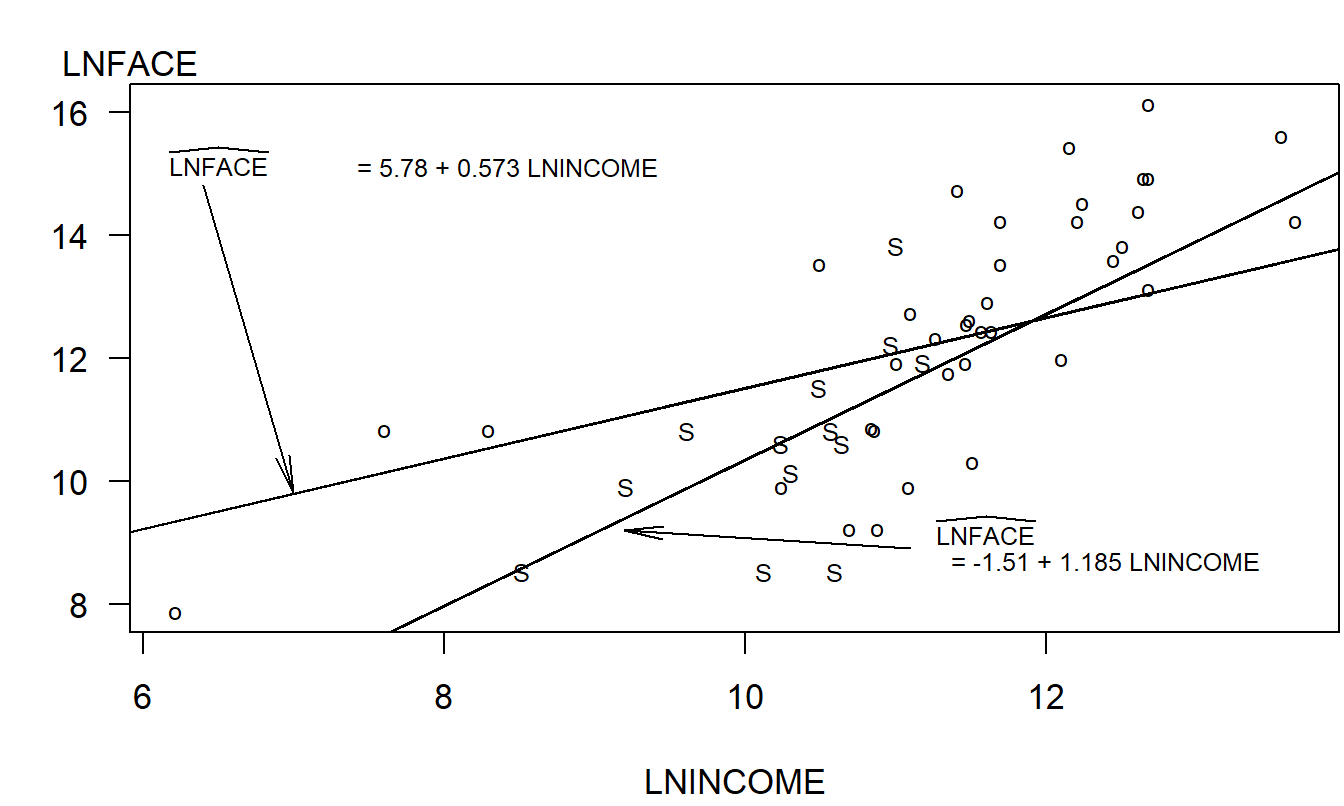
Figure 3.7: Letter plot of LNFACE versus LNINCOME, with the letter code S for single and o for other. The fitted regression lines have been superimposed. The lower line is for single and the upper line is for other.
Example: Life Insurance Company Expenses. In a well-developed life insurance industry, minimizing expenses is critical for a company’s competitive position. Segal (2002) analyzed annual accounting data from over 100 firms for the period 1995-1998, inclusive, using a database from the National Association of Insurance Commissioners (NAIC) and other reported information. Segal modeled overall company expenses as a function of firm outputs and the price of inputs. The outputs consist of insurance production, measured by \(x_1\) through \(x_5\), described in Table 3.10. Segal also considered the square of each output, as well as an interaction term with a dummy/binary variable \(D\) that indicates whether or not the firm uses a branch company to distribute its products. (In a branch company, field managers are company employees, not independent agents.)
Table 3.10.Twenty-Three Regression Coefficients from an Expense Cost Model
\[ \small{ \begin{array}{l|rrrr} \hline & \text{Variable} & &\text{Variable}&\text{ Squared} \\ & \text{Baseline} & \text{Interaction} & \text{Baseline} & \text{Interaction} \\ & & \text{with}~~ & & \text{with}~~ \\ \text{Variable} & (D=0) & (D=1) & (D=0) & (D=1)\\ \hline \text{Number of Life Policies Issued } (x_1) & -0.454 & 0.152 & 0.032 & -0.007 \\ \text{Amount of Term Life Insurance Sold } (x_2) & 0.112 & -0.206 & 0.002 & 0.005 \\ \text{Amount of Whole Life Insurance Sold } (x_3) & -0.184 & 0.173 & 0.008 & -0.007 \\ \text{Total Annuity Considerations } (x_4) & 0.098 & -0.169 & -0.003 & 0.009 \\ \text{Total Accident and Health Premiums } (x_5) &-0.171 & 0.014 & 0.010 & 0.002 \\ \text{Intercept } & 7.726 & & & \\ \text{Price of Labor (PL)} & 0.553 & & & \\ \text{Price of Capital (PC)} & 0.102 & & & \\ \hline \end{array} \\ \begin{array}{l} \textit{Note: } x_1 \text{ through } x_5 \text{ are in logarithmic units}.\\ \textit{Source: Segal (2002)} \end{array} } \]
For the price inputs, the price of labor (\(PL\)) is defined to be the total cost of employees and agents divided by their number, in logarithmic units. The price of capital (\(PC\)) is approximated by the ratio of capital expense to the number of employees and agents, also in logarithmic units. The price of materials consists of expenses other than labor and capital divided by the number of policies sold and terminated during the year. It does not appear directly as an explanatory variable. Rather, Segal took the dependent variable (\(y\)) to be total company expenses divided by the price of materials, again in logarithmic units.
With these variable definitions, Segal estimated the following regression function:
\[ \mathrm{E~}y=\beta_0 + \sum_{j=1}^5 \left( \beta_j x_j + \beta_{j+5} D x_j + \beta_{j+10} x_j^2 + \beta_{j+15}D x_j^2 \right) + \beta_{21} PL + \beta_{22} PC. \]
The parameter estimates appear in Table 3.10. For example, the marginal change in \(\mathrm{E}~y\) per unit change in \(x_1\) is:
\[ \frac{\partial ~ \mathrm{E}~y}{\partial x_1}= \beta_1 + \beta_{6} D + 2 \beta_{11} x_1 + 2 \beta_{16}D x_1, \]
which is estimated as \(-0.454 + 0.152 D + (0.064 - 0.014 D) x_1\). For these data, the median number of policies issued was \(x_1=15,944\). At this value of \(x_1\), the estimated marginal change is \(-0.454 + 0.152 D + (0.064 - 0.014 D) \mathrm{ln}(15944) = 0.165 + 0.017 D,\) or 0.165 for baseline \((D=0)\) and 0.182 for branch \((D=1)\) companies.
These estimates are elasticities, as defined in Section 3.2.2. To interpret these coefficients further, let \(COST\) represent total general company expenses and \(NUMPOL\) represent the number of life policies issued. Then, for branch \((D=1)\) companies, we have:
\[ 0.182 \approx \frac{\partial y }{\partial x_1 } = \frac{\partial ~ \mathrm{ln}~COST}{\partial ~ \mathrm{ln}~NUMPOL}= \frac{ \frac{\partial ~ COST}{\partial ~NUMPOL}} {\frac{COST}{NUMPOL}}, \]
or \(\frac{\partial ~ COST}{\partial ~NUMPOL} \approx 0.182 \frac{COST}{NUMPOL}\). The median cost is $15,992,000, so the marginal cost per policy at these median values is \(0.182 \times (15992000/15944) = \$182.55\).
Special Case: Curvilinear Response Functions
We can expand the polynomial functions of an explanatory variable to include several explanatory variables. For example, the expected response, or response function, for a second-order model with two explanatory variables is:
\[ \mathrm{E} y = \beta_0 + \beta_1 x_1 + \beta_2 x_2 + \beta_{11} x_1^2 + \beta_{22} x_2^2 + \beta_{12} x_1 x_2. \]
Figure 3.8 illustrates this response function. Similarly, the response function for a second-order model with three explanatory variables is:
\[ \mathrm{E} y = \beta_0 + \beta_1 x_1 + \beta_2 x_2 + \beta_3 x_3 + \beta_{11} x_1^2 + \beta_{22} x_2^2 + \beta_{33} x_3^2 + \beta_{12} x_1 x_2 + \beta_{13} x_1 x_3 + \beta_{23} x_2 x_3. \]
When there is more than one explanatory variable, third and higher-order models are rarely used in applications.
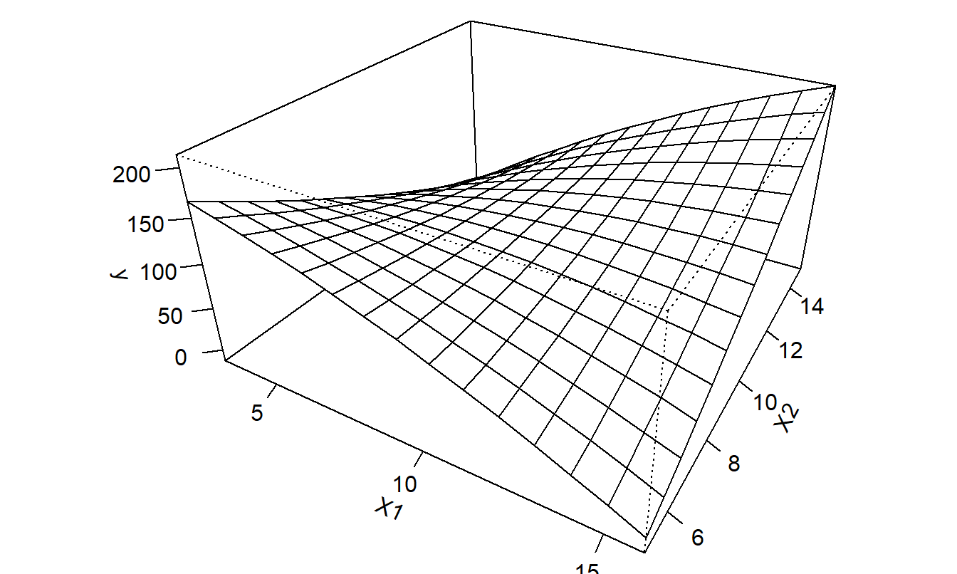
Figure 3.8: Plot of \(\mathrm{E}~y = \beta_0 + \beta_1~x_1 + \beta_2~x_2 + \beta_{11}~x_1^2 + \beta_{22}~x_2^2 + \beta_{12}~x_1~x_2\) versus \(x_1\) and \(x_2\).
R Code to Produce Figure 3.8
Special Case: Nonlinear Functions of a Continuous Variable
In some applications, we expect the response to have some abrupt changes in behavior at certain values of an explanatory variable, even if the variable is continuous. For example, suppose that we are trying to model an individual’s charitable contributions (\(y\)) in terms of their wages (\(x\)). For 2007 data, a simple model we might entertain is given in Figure 3.9.
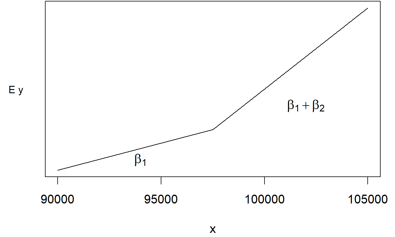
Figure 3.9: The marginal change in \(\mathrm{E}~y\) is lower below $97,500. The parameter \(\beta_2\) represents the difference in the slopes.
R Code to Produce Figure 3.9
A rationale for this model is that, in 2007, individuals paid 7.65% of their income for Social Security taxes up to 97,500. No Social Security taxes are excised on wages in excess of 97,500. Thus, one theory is that, for wages in excess of $97,500, individuals have more disposable income per dollar and thus should be more willing to make charitable contributions.
To model this relationship, define the binary variable \(z\) to be zero if \(x < 97,500\) and to be one if \(x \ge 97,500\). Define the regression function to be \(\mathrm{E}~y = \beta_0 + \beta_1 x + \beta_2 z (x - 97,500)\). This can be written as:
\[ \mathrm{E}~y = \begin{cases} \beta_0 + \beta_1 x & x < 97,500 \\ \beta_0 - \beta_2(97,500) + (\beta_1+\beta_2) x & x \geq 97,500 \end{cases} \]
To estimate this model, we would run a regression of \(y\) on two explanatory variables, \(x_1 = x\) and \(x_2 = z \times (x - 97,500)\). If \(\beta_2 > 0\), then the marginal rate of charitable contributions is higher for incomes exceeding $97,500.
Figure 3.9 illustrates this relationship, known as piecewise linear regression or sometimes a “broken stick” model. The sharp break in Figure 3.9 at \(x = 97,500\) is called a “kink.” We have linear relationships above and below the kinks and have used a binary variable to put the two pieces together. We are not restricted to one kink. For example, suppose that we wish to do a historical study of Federal taxable income for 1992 single filers. Then, there were three tax brackets: the marginal tax rate below 21,450 was 15%, above 51,900 was 31%, and in between was 28%. For this example, we would use two kinks, at 21,450 and 51,900.
Further, piecewise linear regression is not restricted to continuous response functions. For example, suppose that we are studying the commissions paid to stockbrokers (\(y\)) in terms of the number of shares purchased by a client (\(x\)). We might expect to see the relationship illustrated in Figure 3.10. Here, the discontinuity at \(x = 100\) reflects the administrative expenses of trading in odd lots, as trades of less than 100 shares are called. The lower marginal cost for trades in excess of 100 shares simply reflects the economies of scale for doing business in larger volumes. A regression model of this is \(\mathrm{E}~y = \beta_0 + \beta_1 x + \beta_2 z + \beta_3 z x\) where \(z = 0\) if \(x < 100\) and \(z = 1\) if \(x \geq 100\). The regression function depicted in Figure 3.10 is:
\[ \mathrm{E}~y = \begin{cases} \beta_0 + \beta_1 x_1 & x < 100 \\ \beta_0 + \beta_2 + (\beta_1+\beta_3) x_1 & x \geq 100 \end{cases} \]
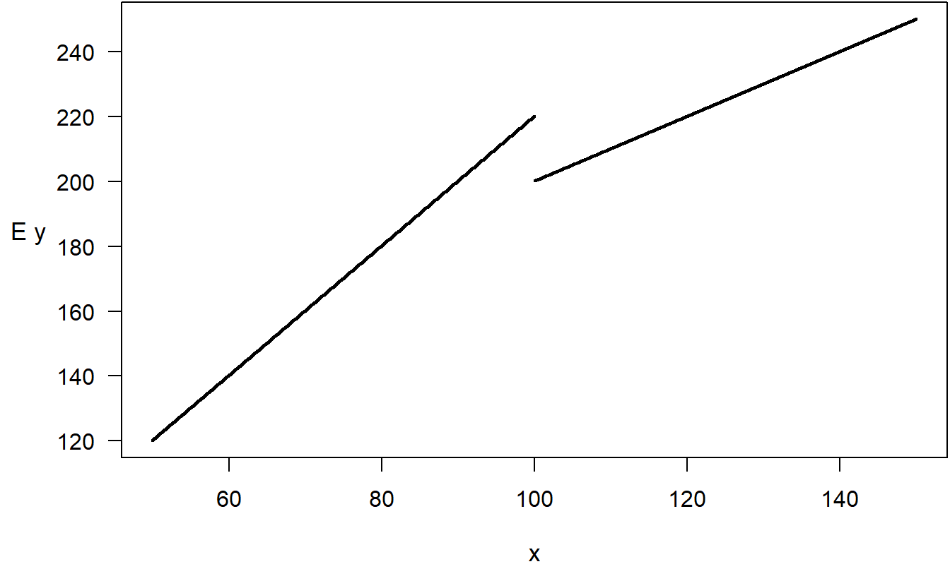
Figure 3.10: Plot of expected commissions (\(\mathrm{E}~y\)) versus number of shares traded (\(x\)). The break at \(x=100\) reflects savings in administrative expenses. The lower slope for \(x \ge 100\) reflects economies of scales in expenses.
R Code to Produce Figure 3.10
Video: Section Summary
3.6 Further Reading and References
For proofs of the Chapter 3 results, we refer the reader to Goldberger (1991). Nonlinear regression models are discussed in, for example, Bates and Watts (1988).
Chapter 3 has introduced the fundamentals of multiple linear regression. Chapter 4 will widen the scope by introducing categorical variables and statistical inference methods for handling several coefficients simultaneously. Chapter 5 will introduce techniques to help you pick appropriate variables in a multiple linear regression model. Chapter 6 is a synthesis chapter, discussing model interpretation, variable selection and data collection.
Chapter References
- Bates, Douglas M. and Watts, D. G. (1988). Nonlinear Regression Analysis and its Applications. John Wiley & Sons, New York.
- Lemaire, Jean (2002). Why do females live longer than males? North American Actuarial Journal, 6(4), 21-37.
- Goldberger, Arthur (1991). A Course in Econometrics. Harvard University Press, Cambridge.
- Plackett, R.L. (1960). Regression Analysis. Clarendon Press, Oxford, England.
- Segal, Dan (2002). An economic analysis of life insurance company expenses. North American Actuarial Journal, 6(4), 81-94.
3.7 Exercises
3.1. Consider a fictitious data set of \(n = 100\) observations with \(s_y = 100\). We run a regression with three explanatory variables to get \(s = 50\).
- Calculate the adjusted coefficient of determination, \(R_a^2\).
- Complete the ANOVA table.
\[ \small{ \begin{array}{|l|l|c|l|} \hline \text{ANOVA Table} \\ \hline \text{Source} & \text{Sum of Squares} & \text{df} & \text{Mean Square} \\ \hline \text{Regression} & & & \\ \text{Error} & & & \\ \text{Total} & & & \\ \hline \end{array} } \] c. Calculate the (unadjusted) coefficient of determination, \(R^2\).
3.2. Consider a fictitious data set of \(n = 100\) observations with \(s_y = 80\). We run a regression with three explanatory variables to get \(s = 50\). We also get
\[ \small{ \left(\mathbf{X^{\prime} X} \right)^{-1} = \begin{pmatrix} 100 & 20 & 20 & 20 \\ 20 & 90 & 30 & 40 \\ 20 & 30 & 80 & 50 \\ 20 & 40 & 50 & 70 \\ \end{pmatrix}. } \]
- Determine the standard error of \(b_3\), \(se(b_3)\).
- Determine the estimated covariance between \(b_2\) and \(b_3\).
- Determine the estimated correlation between \(b_2\) and \(b_3\).
- Determine the estimated variance of \(4b_2 + 3b_3\).
3.3. Consider the following small fictitious data set. You will be fitting a regression model to \(y\) using two explanatory variables, \(x_1\) and \(x_2\).
\[ \small{ \begin{array}{c|cccc} \hline i & 1 & 2 & 3 & 4 \\ \hline x_{i,1} & -1 & 2 & 4 & 6 \\ x_{i,2} & 0 & 0 & 1 & 1 \\ y_i & 0 & 1 & 5 & 8 \\ \hline \end{array} } \]
From the fitted regression model, we have \(s = 1.373\) and \[ \small{ \mathbf{b} = \begin{pmatrix} 0.1538 \\ 0.6923 \\ 2.8846 \end{pmatrix} ~~~\text{and}~~~ \left(\mathbf{X^{\prime} X} \right)^{-1} = \begin{pmatrix} 0.53846 & -0.07692 & -0.15385 \\ -0.07692 & 0.15385 & -0.69231 \\ -0.15385 & -0.69231 & 4.11538 \\ \end{pmatrix}. } \]
- Write down the vector of dependent variables, \(\mathbf{y}\), and the matrix of explanatory variables, \(\mathbf{X}\).
- Determine the numerical value for \(\widehat{y}_3\), the fitted value for the third observation.
- Determine the numerical value for \(se(b_2)\).
- Determine the numerical value for \(t(b_1)\).
3.4. Wisconsin Lottery. Section 2.1 described a sample of \(n=50\) geographic areas (zip codes) containing sales data on the Wisconsin state lottery (\(y = \text{SALES}\)). In that section, sales were analyzed using a basic linear regression model with \(x = \text{POP}\), the area population, as the explanatory variable. This exercise extends that analysis by introducing additional explanatory variables given in Table 3.11.
\[ \text{Table 3.11: Lottery, economic and demographic characteristics of fifty Wisconsin ZIP codes} \]
\[ \small{ \begin{array}{ll} \hline \textbf{Lottery characteristics} \\ \hline \text{SALES} & \text{Online lottery sales to individual consumers} \\ \hline \textbf{Economic and } \\ ~~~~~\textbf{demographic characteristics} \\\hline \text{PERPERHH} & \text{Persons per household} \\ \text{MEDSCHYR} & \text{Median years of schooling} \\ \text{MEDHVL} & \text{Median home value in \$1000s for owner-occupied homes} \\ \text{PRCRENT} & \text{Percent of housing that is renter occupied} \\ \text{PRC55P} & \text{Percent of population that is 55 or older} \\ \text{HHMEDAGE} & \text{Household median age} \\ \text{MEDINC} & \text{Estimated median household income, in \$1000s} \\ \text{POP} & \text{Population} \\ \hline \end{array} } \]
- Produce a table of summary statistics for all variables. One zip code (observation 11, zip = 53211, Shorewood Wisconsin, a suburb of Milwaukee) appears to have unusually large values of MEDSCHYR and MEDHVL. For this observation, how many standard deviations is the value of MEDSCHYR above the mean? For this observation, how many standard deviations is the value of MEDHVL above the mean?
- Produce a table of correlations. What three variables are most highly correlated with SALES?
- Produce a scatter plot matrix of all explanatory variables and SALES. In the plot of MEDSCHYR versus SALES, describe the position of observation 11.
- Fit a linear model of SALES on all eight explanatory variables. Summarize the fit of this model by citing the residual standard deviation, \(s\), the coefficient of determination, \(R^2\) and its adjusted version, \(R_a^2\).
- Based on your part (d) model fit, is MEDSCHYR a statistically significant variable? To respond to this question, use a formal test of hypothesis. State your null and alternative hypotheses, decision-making criterion and your decision-making rule.
- Now fit a more parsimonious model, using SALES as the dependent variable and MEDSCHYR, MEDHVL and POP as explanatory variables. Summarize the fit of this model by citing the residual standard deviation, \(s\), the coefficient of determination, \(R^2\) and its adjusted version, \(R_a^2\). How do these values compare to the model fit in part (d)?
- Note that the sign of the regression coefficient associated with MEDSCHYR is negative. To help interpret this coefficient, compute the corresponding partial correlation coefficient. What is the interpretation of this coefficient?
- To get further insights into the relation between MEDSCHYR and SALES, produce an added variable plot controlling for the effects of MEDHVL and POP. Check that the correlation associated with this plot agrees with your answer in part (g).
- Re-run the regression in part (f), after removing observation 11. Cite the basic summary statistics from this regression. For this model fit, is MEDSCHYR a statistically significant variable? To respond to this question, use a formal test of hypothesis. State your null and alternative hypotheses, decision-making criterion and your decision-making rule.
- Re-run the regression in part (f), after removing observation 9. Cite the basic summary statistics from this regression.
3.5. Insurance Company Expenses. This exercise considers insurance company data from the NAIC and described in Exercise 1.
Table 3.10 describes several variables that can be used to explain expenses. As with Segal’s (2002) study of life insurers, firm “outputs” consist of premiums written (for property and casualty, these are subdivided into personal and commercial lines) as well as losses (subdivided into short and long tail lines). ASSETS and CASH are commonly used measures of the size of a company. GROUP, STOCK, and MUTUAL describe the organizational structure. Firm “inputs” were gathered from the Bureau of Labor Statistics (BLS, from the Occupational Employee Statistics program). STAFFWAGE is calculated as the average wage in the state where the insurance company is headquartered. AGENTWAGE is calculated as the weighted average of annual wages of the brokerage industry, weighted by the percentage of gross premium written in each state.
| Variable | Description |
|---|---|
| EXPENSES | Total expenses incurred, in millions of dollars |
| LONGLOSS | Losses incurred for long tail lines, in millions of dollars |
| SHORTLOSS | Losses incurred for short tail lines, in millions of dollars |
| GPWPERSONAL | Gross premium written for personal lines, in millions of dollars |
| GPWCOMM | Gross premium written for commercial lines, in millions of dollars |
| ASSETS | Net admitted assets, in millions of dollars |
| CASH | Cash and invested assets, in millions of dollars |
| GROUP | Indicates if the company is affiliated |
| STOCK | Indicates if the company is a stock company |
| MUTUAL | Indicates if the company is a mutual company |
| STAFFWAGE | Annual average wage of the insurer’s administrative staff, in thousands of dollars |
| AGENTWAGE | Annual average wage of the insurance agent, in thousands of dollars |
A preliminary inspection of the data showed that many firms did not report any insurance losses incurred in 2005. For this exercise, we consider the 384 companies with some losses in the file NAICExpense.csv.
Summary Statistics
Produce summary statistics of the response variable and the (non-binary) explanatory variables. Note the pattern of skewness for each variable. Note that many variables have negative values.Transform Variables
Transform each non-binary variable through the modified logarithm transform, \(\ln(1+x)\). Produce summary statistics of these modified non-binary explanatory variables. Let LNEXPENSES (\(= \ln(1+\text{EXPENSES})\)) denote the modified expense variable.
For subsequent analysis, use only the modified variables described in part (b).Correlation Table
Produce a table of correlations for the non-binary variables. What three variables are most highly correlated with LNEXPENSES?Boxplot of LNEXPENSES by GROUP
Provide a boxplot of LNEXPENSES by level of GROUP. Which level of group has higher expenses?Linear Model on All Variables
Fit a linear model of LNEXPENSES on all eleven explanatory variables. Summarize the fit of this model by citing the residual standard deviation, \(s\), the coefficient of determination, \(R^2\), and its adjusted version, \(R^2_a\).Reduced Model
Fit a linear model of LNEXPENSES on a reduced model using eight explanatory variables, dropping LNCASH, STOCK, and MUTUAL. For the explanatory variables, include ASSETS, GROUP, both versions of losses, and gross premiums, as well as the two BLS variables.f(i). Summarize the fit of this model by citing \(s\), \(R^2\), and \(R^2_a\).
f(ii). Interpret the coefficient associated with commercial lines gross premiums on the logarithmic scale.
f(iii). Suppose that GPWCOMM increases by $1, how much do we expect EXPENSES to increase? Use your answer in part f(ii) and median values of GPWCOMM and EXPENSES for this question.Quadratic Terms
Square each of the two loss and the two gross premium variables. Fit a linear model of LNEXPENSES on a reduced model using twelve explanatory variables, the eight variables in part (f) and the four additional squared terms just created.
g(i). Summarize the fit of this model by citing \(s\), \(R^2\), and \(R^2_a\).
g(ii). Do the quadratic variables appear to be useful explanatory variables?Excluding BLS Variables
Now omit the two BLS variables, so you are fitting a model of LNEXPENSES on ASSETS, GROUP, both versions of losses, and gross premiums, as well as quadratic terms. Summarize the fit of this model by citing \(s\), \(R^2\), and \(R^2_a\). Comment on the number of observations used to fit this model compared to part (f).Interaction Terms
Drop the quadratic terms in part (g) and add interaction terms with the dummy variable GROUP. Thus, there are now eleven variables: ASSETS, GROUP, both versions of losses and gross premiums, as well as interactions of GROUP with ASSETS and both versions of losses and gross premiums.
i(i). Summarize the fit of this model by citing \(s\), \(R^2\), and \(R^2_a\).
i(ii). Suppose that GPWCOMM increases by $1, how much do we expect EXPENSES to increase for GROUP=0 companies? Use the median values of GPWCOMM and EXPENSES of GROUP=0 companies for this question.
i(iii). Suppose that GPWCOMM increases by $1, how much do we expect EXPENSES to increase for GROUP=1 companies? Use the median values of GPWCOMM and EXPENSES of GROUP=1 companies for this question.
3.6 National Life Expectancies. We continue the analysis begun in Exercises 1 and 2. Now fit a regression model on LIFEEXP using three explanatory variables: FERTILITY, PUBLICEDUCATION, and lnHEALTH (the natural logarithmic transform of PRIVATEHEALTH).
- Interpretation of Public Education Coefficient
Interpret the regression coefficient associated with PUBLICEDUCATION. - Interpretation of Health Expenditures Coefficient
Interpret the regression coefficient associated with HEALTH expenditures without using the logarithmic scale for expenditures. - Statistical Significance of PUBLICEDUCATION
Based on the model fit, is PUBLICEDUCATION a statistically significant variable? To respond to this question, use a formal test of hypothesis. State your null and alternative hypotheses, decision-making criterion, and your decision-making rule. - Added Variable Plot
The negative sign of the PUBLICEDUCATION coefficient is surprising, given that the sign of the correlation between PUBLICEDUCATION and LIFEEXP is positive and intuition suggests a positive relation. To check this result, an added variable plot appears in Figure 3.11.
d(i). For an added variable plot, describe its purpose and a method for producing it.
d(ii). Calculate the correlation corresponding to the added variable plot that appears in Figure 3.11.
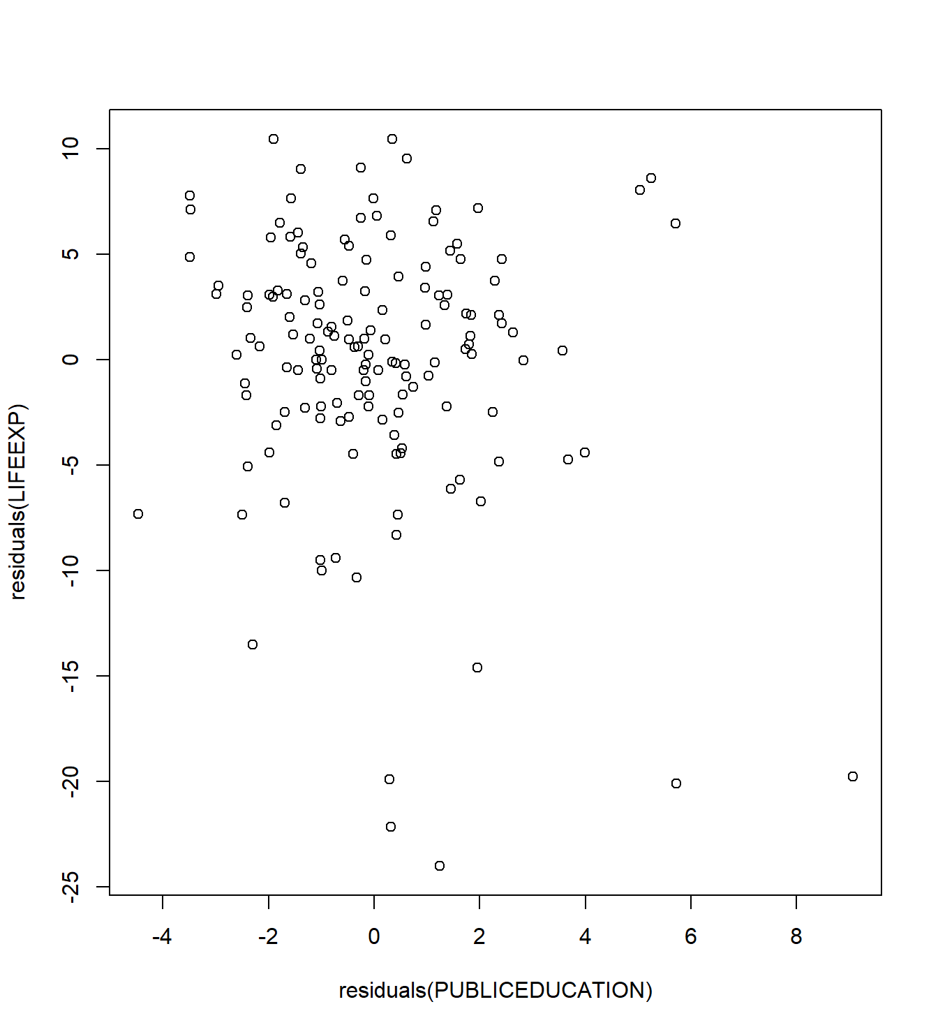
Figure 3.11: Added variable plot of PUBLICEDUCATION versus LIFEEXP, controlling for FERTILITY and lnHEALTH