Chapter 16 Frequency-Severity Models
Chapter Preview. Many data sets feature dependent variables that have a large proportion of zeros. This chapter introduces a standard econometric tool, known as a tobit model, for handling such data. The tobit model is based on observing a left-censored dependent variable, such as sales of a product or claim on a healthcare policy, where it is known that the dependent variable cannot be below zero. Although this standard tool can be useful, many actuarial data sets that feature a large proportion of zeros are better modeled in “two parts,” one part for the frequency and one part for the severity. This chapter introduces two-part models and provides extensions to an aggregate loss model, where a unit under study, such as an insurance policy, can result in more than one claim.
16.1 Introduction
Many actuarial data sets come in “two parts:”
- One part for the frequency, indicating whether or not a claim has occurred or, more generally, the number of claims, and
- One part for the severity, indicating the amount of a claim.
In predicting or estimating claims distributions, we often associate the cost of claims with two components: the event of the claim and its amount, if the claim occurs. Actuaries term these the claims frequency and severity components, respectively. This is the traditional way of decomposing “two-part” data, where one can think of a zero as arising from a policy without a claim (Bowers et al., 1997, Chapter 2). Because of this decomposition, two-part models are also known as frequency-severity models. However, this formulation has been traditionally used without covariates to explain either the frequency or severity components. In the econometrics literature, Cragg (1971) introduced covariates into these two components, citing an example from fire insurance.
Healthcare data also often feature a large proportion of zeros that must be accounted for in the modeling. Zero values can represent an individual’s lack of healthcare utilization, no expenditure, or non-participation in a program. In healthcare, Mullahy (1998) cites some prominent areas of potential applicability:
- Outcomes research - amount of health care utilization or expenditures
- Demand for health care - amount of health care sought, such as the number of physician visits
- Substance abuse - amount consumed of tobacco, alcohol, and illicit drugs.
The two-part aspect can be obscured by a natural way of recording data; enter the amount of the claim when the claim occurs (a positive number) and a zero for no claim. It is easy to overlook a large proportion of zeros, particularly when the analyst is also concerned with many covariates that may help explain a dependent variable. As we will see in this chapter, ignoring the two-part nature can lead to serious bias. To illustrate, recall from Chapter 6 a plot of an individual’s income (\(x\)) versus the amount of insurance purchased (\(y\)) (Figure 6.3). Fitting a single line to these data would misinform users about the effects of \(x\) on \(y\).
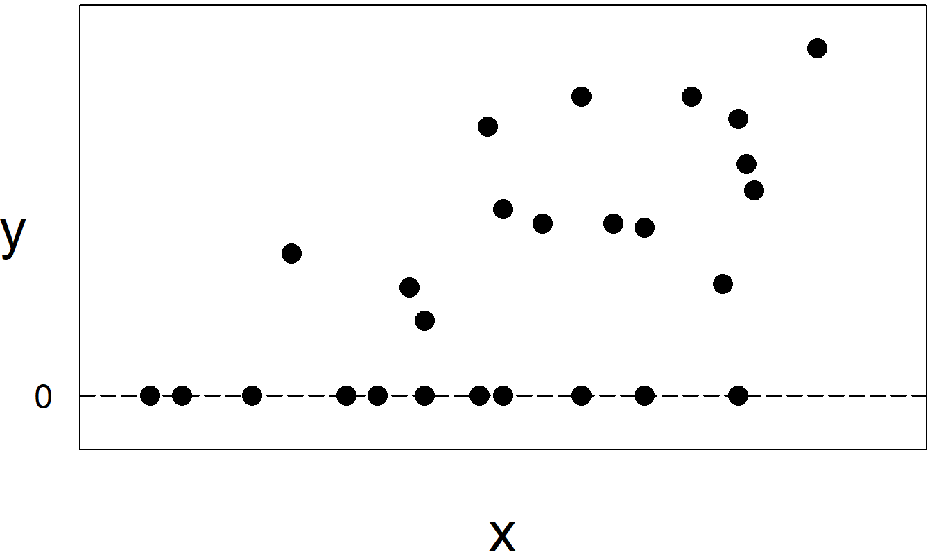
Figure 16.1: When individuals do not purchase insurance, they are recorded as \(y=0\) sales. The sample in this plot represents two subsamples, those who purchased insurance, corresponding to \(y>0\), and those who did not, corresponding to \(y=0\).
In contrast, many insurers keep separate data files for frequency and severity. For example, insurers maintain a “policyholder” file that is established when a policy is underwritten. This file records much underwriting information about the insured(s), such as age, gender, and prior claims experience, policy information such as coverage, deductibles, and limitations, as well as the insurance claims event. A separate file, often known as the “claims” file, records details of the claim against the insurer, including the amount. (There may also be a “payments” file that records the timing of the payments although we shall not deal with that here.) This recording process makes it natural for insurers to model the frequency and severity as separate processes.
16.2 Tobit Model
One way of modeling a large proportion of zeros is to assume that the dependent variable is (left) censored at zero. This chapter introduces left-censored regression, beginning with the well-known tobit model that is based on the pioneering work of James Tobin (1958). Subsequently, Goldberger (1964) coined the phrase “tobit model,” acknowledging the work of Tobin and its similarity to the probit model.
As with probit (and other binary response) models, we use an unobserved, or latent, variable \(y^{\ast}\) that is assumed to follow a linear regression model of the form \[ y_i^{\ast} = \mathbf{x}_i^{\prime} \boldsymbol{\beta} + \varepsilon_i. \tag{16.1} \] The responses are censored or “limited” in the sense that we observe \(y_i = \max \left( y_i^{\ast},d_i\right)\). The limiting value, \(d_i\), is a known amount. Many applications use \(d_i=0\), corresponding to zero sales or expenses, depending on the application. However, we also might use \(d_i\) for the daily expenses claimed for travel reimbursement and allow the reimbursement (such as 50 or 100) to vary by employee \(i\). Some readers may wish to review Section 14.2 for an introduction to censoring.
The model parameters consist of the regression coefficients, \(\boldsymbol{\beta}\), and the variability term, \(\sigma^2 = \mathrm{Var}~\varepsilon_i\). With equation (16.1), we interpret the regression coefficients as the marginal change of \(\mathrm{E~}y^{\ast}\) per unit change in each explanatory variable. This may be satisfactory in some applications, such as when \(y^{\ast}\) represents an insurance loss. However, for most applications, users are typically interested in marginal changes in \(\mathrm{E~}y\), that is, the expected value of the observed response.
To interpret these marginal changes, it is customary to adopt the assumption of normality for the latent variable \(y_i^{\ast}\) (or equivalently for the disturbance \(\varepsilon_i\)). With this assumption, standard calculations (see Exercise 16.1) show that \[ \mathrm{E~}y_i = d_i + \Phi \left( \frac{\mathbf{x}_i^{\prime} \boldsymbol{\beta} - d_i}{\sigma}\right) \left( \mathbf{x}_i^{\prime} \boldsymbol{\beta} - d_i + \sigma \lambda_i\right), \tag{16.2} \] where \[ \lambda_i = \frac{\mathrm{\phi}\left( \left(\mathbf{x}_i^{\prime} \boldsymbol{\beta} - d_i\right)/\sigma \right)}{\Phi\left( \left(\mathbf{x}_i^{\prime} \boldsymbol{\beta} - d_i\right)/\sigma \right)}. \] Here, \(\mathrm{\phi}(\cdot)\) and \(\Phi(\cdot)\) are the standard normal density and distribution functions, respectively. The ratio of a probability density function to a cumulative distribution function is sometimes called an inverse Mills ratio. Although complex in appearance, equation (16.2) allows one to readily compute \(\mathrm{E~} y\). For large values of \(\left(\mathbf{x}_i^{\prime}\boldsymbol{\beta} - d_i\right)/\sigma\), we see that \(\lambda_i\) is close to 0 and \(\Phi\left( \left(\mathbf{x}_i^{\prime}\boldsymbol{\beta} - d_i\right)/\sigma \right)\) is close to 1. We interpret this to mean, for large values of the systematic component \(\mathbf{x}_i^{\prime}\boldsymbol{\beta}\), that the regression function \(\mathrm{E~}y_i\) tends to be linear and the usual interpretations apply. The tobit model specification has the greatest impact on observations close to the limiting value \(d_i\).
Equation (16.2) shows that if an analyst ignores the effects of censoring, then the regression function can be quite different than the typical linear regression function, \(\mathrm{E~}y=\mathbf{x}^{\prime}\boldsymbol{\beta}\), resulting in biased estimates of coefficients. The other tempting path is to exclude limited observations (\(y_i=d_i\)) from the dataset and again run ordinary regression. However, standard calculations also show that
\[ \mathrm{E~}\left( y_i|\ y_i>d_i\right) =\mathbf{x}_i^{\prime}\boldsymbol{\beta} + \sigma \frac{\mathrm{\phi}\left( (\mathbf{x}_i^{\prime} \boldsymbol{\beta} - d_i)/\sigma \right)}{1-\Phi \left( (\mathbf{x}_i^{\prime} \boldsymbol{\beta} - d_i)/\sigma \right)} \tag{16.3} \]
Thus, this procedure also results in biased regression coefficients.
A commonly used method of estimating the tobit model is maximum likelihood. Employing the normality assumption, standard calculations show that the log-likelihood can be expressed as
\[ \begin{array}{ll} \ln L &= \sum\limits_{i:y_i=d_i} \ln \left\{ 1-\Phi \left( \frac{\mathbf{x}_i^{\prime}\boldsymbol{\beta} - d_i}{\sigma}\right) \right\} \\ & - \frac{1}{2} \sum\limits_{i:y_i>d_i} \left\{ \ln 2\pi \sigma^2 + \frac{(y_i-(\mathbf{x}_i^{\prime}\boldsymbol{\beta}-d_i))^2}{\sigma^2}\right\}, \tag{16.4} \end{array} \]
where \(\{i:y_i=d_i\}\) and \(\{i:y_i>d_i\}\) means the sum over the censored and noncensored observations, respectively. Many statistical software packages can readily compute the maximum likelihood estimators, \(\mathbf{b}_{MLE}\) and \(s_{MLE}\), as well as corresponding standard errors. Section 11.9 introduces likelihood inference.
For some users, it is convenient to have an algorithm that does not rely on specialized software. A two-stage algorithm due to Heckman (1976) fulfills this need. For this algorithm, first subtract \(d_i\) from each \(y_i\), so that one may take \(d_i\) to be zero without loss of generality. Even for those who wish to use the more efficient maximum likelihood estimators, Heckman’s algorithm can be useful in the model exploration stage as one uses linear regression to help select the appropriate form of the regression equation.
Heckman’s Algorithm for Estimating Tobit Model Parameters
For the first stage, define the binary variable \[ r_i=\left\{ \begin{array}{ll} 1 & \text{if } y_i>0 \\ 0 & \text{if } y_i=0 \end{array} \right. , \] indicating whether or not the observation is censored. Run a probit regression using \(r_i\) as the dependent variable and \(\mathbf{x}_i\) as explanatory variables. Call the resulting regression coefficients \(\mathbf{g}_{PROBIT}\).
For each observation, compute the estimated variable \[ \widehat{\lambda}_i=\frac{\mathrm{\phi }\left( \mathbf{x}_i^{\prime} \mathbf{g}_{PROBIT}\right) }{\Phi \left( \mathbf{x}_i^{\prime} \mathbf{g}_{PROBIT}\right) }, \] an inverse Mill’s ratio. With this, run a regression of \(y_i\) on \(\mathbf{x}_i\) and \(\widehat{\lambda}_i\). Call the resulting regression coefficients \(\mathbf{b}_{2SLS}\).
The idea behind this algorithm is that equation (16.1) has the same form as the probit model; thus, consistent estimates of the regression coefficients (up to scale) can be computed. The regression coefficients \(\mathbf{b}_{2SLS}\) provide consistent and asymptotically normal estimates of \(\boldsymbol{\beta}\). They are, however, inefficient compared to the maximum likelihood estimators, \(\mathbf{b}_{MLE}\). Standard calculations (see Exercise 16.1) show that \(\mathrm{Var~}\left( y_i|\ y_i>d_i\right)\) depends on \(i\) (even when \(d_i\) is constant). Thus, it is customary to use heteroscedasticity-consistent standard errors for \(\mathbf{b}_{2SLS}\).
16.3 Application: Medical Expenditures
This section considers data from the Medical Expenditure Panel Survey (MEPS) that were introduced in Section 11.4. Recall that MEPS is a probability survey that provides nationally representative estimates of health care use, expenditures, sources of payment, and insurance coverage for the U.S. civilian population. We consider MEPS data from the first panel of 2003 and take a random sample of \(n=2,000\) individuals between ages 18 and 65. Section 11.4 analyzed the frequency component, trying to understand the determinants that influenced whether or not people were hospitalized. Section 13.4 analyzed the severity component; given that a person was hospitalized, what are the determinants of medical expenditures? This chapter seeks to unify these two components into a single model of healthcare utilization.
Summary Statistics
Table 16.1 reviews these explanatory variables and provides summary statistics that suggest their effects on expenditures of inpatient visits. The second column, “Average Expend,” displays the average logarithmic expenditure by explanatory variable, treating no expenditures as a zero (logarithmic) expenditure. This would be the primary variable of interest if one did not decompose the total expenditure into a discrete zero and continuous amount.
Examining this overall average (logarithmic) expenditure, we see that females had higher expenditures than males. In terms of ethnicity, Native Americans and Asians had the lowest average expenditures. However, these two ethnic groups accounted for only 5.4% of the total sample size. Regarding regions, it appears that individuals from the West had the lowest average expenditures. In terms of education, more educated persons had lower expenditures. This observation supports the theory that more educated persons take more active roles in keeping their health. When it comes to self-rated health status, poorer physical, mental health, and activity-related limitations led to greater expenditures. Lower-income individuals had greater expenditures, and those with insurance coverage had greater average expenditures.
Table 16.1 also describes the effects of explanatory variables on the frequency of utilization and average expenditures for those that used inpatient services. As in Table 11.4, the column “Percent Positive Expend” gives the percentage of individuals that had some positive expenditure, by explanatory variable. The column “Average of Pos Expend” gives the average (logarithmic) expenditure in cases where there was an expenditure, ignoring the zeros. This is comparable to the median expenditure in Table 13.5 (given in dollars, not log dollars).
To illustrate, consider that females had higher average expenditures than males by looking at the “Average Expend” column. Breaking this down into frequency and amount of utilization, we see that females had a higher frequency of utilization but, when they had a positive utilization, the average (logarithmic) expenditure was lower than males. An examination of Table 16.1 shows this observation holds true for other explanatory variables. A variable’s effect on overall expenditures may be positive, negative, or non-significant; this effect can be quite different when we decompose expenditures into frequency and amount components.
Table 16.2 compares the ordinary least squares (OLS) regression to maximum likelihood estimates for the tobit model. From this table, we can see that there is a substantial agreement among the \(t\)-ratios for these fitted models. This agreement comes from examining the sign (positive or negative) and the magnitude (such as exceeding two for statistical significance) of each variable’s \(t\)-ratio. The regression coefficients also largely agree in sign. However, it is not surprising that the magnitudes of the regression coefficients differ substantially. This is because, from equation (16.2), we can see that the tobit coefficients measure the marginal change of the expected latent variable \(y^{\ast}\), not the marginal change of the expected observed variable \(y\), as does OLS.
Table 16.1. Percent of Positive Expenditures and Average Logarithmic Expenditure, by Explanatory Variable
\[ \scriptsize{ \begin{array}{lllrrrr}\hline \text{Category} & \text{Variable} & \text{Description} & \text{Percent} & \text{Average} & \text{Percent} & \text{Average} \\ & & & \text{of data} & \text{Expend} & \text{Positive} & \text{of Pos} \\ & & & & & \text{Expend} & \text{Expend} \\ \hline \text{Demography} & AGE & \text{Age in years } \\ & & \ \ \ \text{18 to 65 (mean: 39.0)} \\ & GENDER & \text{1 if female} & 52.7 & 0.91 & 10.7 & 8.53 \\ & GENDER & \text{0 if male} & 47.3 & 0.40 & 4.7 & 8.66 \\ \text{Ethnicity} & ASIAN & \text{1 if Asian} & 4.3 & 0.37 & 4.7 & 7.98 \\ & BLACK & \text{1 if Black} & 14.8 & 0.90 & 10.5 & 8.60 \\ & NATIVE & \text{1 if Native} & 1.1 & 1.06 & 13.6 & 7.79 \\ & WHITE & \text{Reference level} & 79.9 & 0.64 & 7.5 & 8.59 \\ \text{Region} & NORTHEAST & \text{1 if Northeast} & 14.3 & 0.83 & 10.1 & 8.17 \\ & MIDWEST & \text{1 if Midwest} & 19.7 & 0.76 & 8.7 & 8.79 \\ & SOUTH & \text{1 if South} & 38.2 & 0.72 & 8.4 & 8.65 \\ & WEST & \text{Reference level} & 27.9 & 0.46 & 5.4 & 8.51 \\ \hline \text{Education} & COLLEGE & \text{1 if college or higher degree} & 27.2 & 0.58 & 6.8 & 8.50 \\ & HIGHSCHOOL & \text{1 if high school degree} & 43.3 & 0.67 & 7.9 & 8.54 \\ & & \text{Reference level is } & 29.5 & 0.76 & 8.8 & 8.64 \\ & & \ \ \ \text{lower than high school degree} & & & & \\ \hline \text{Self-rated} & POOR & \text{1 if poor} & 3.8 & 3.26 & 36.0 & 9.07 \\ ~~\text{physical health} & FAIR & \text{1 if fair} & 9.9 & 0.66 & 8.1 & 8.12 \\ & GOOD & \text{1 if good} & 29.9 & 0.70 & 8.2 & 8.56 \\ & VGOOD & 1 \text{if very good} & 31.1 & 0.54 & 6.3 & 8.64 \\ & & \text{Reference level is excellent health} & 25.4 & 0.42 & 5.1 & 8.22 \\ \text{Self-rated} & MNHPOOR & \text{1 if poor or fair} & 7.5 & 1.45 & 16.8 & 8.67 \\ ~~\text{mental health} & & \text{0 if good to excellent mental health} & 92.5 & 0.61 & 7.1 & 8.55 \\ \text{Any activit}y & ANYLIMIT & \text{1 if any functional or activity limitation} & 22.3 & 1.29 & 14.6 & 8.85 \\ ~~\text{limitation} & & \text{0 if otherwise} & 77.7 & 0.50 & 5.9 & 8.36 \\ \hline \text{Income compared} & HINCOME & \text{1 if high income} & 31.6 & 0.47 & 5.4 & 8.73 \\ \text{to poverty line} & MINCOME & \text{1 if middle income }& 29.9 & 0.61 & 7.0 & 8.75 \\ & LINCOME & \text{1 if low income} & 15.8 & 0.73 & 8.3 & 8.87 \\ & NPOOR & \text{1 if near poor} & 5.8 & 0.78 & 9.5 & 8.19 \\ & & \text{Reference level is poor/negative }& 17.0 & 1.06 & 13.0 & 8.18 \\ \hline \text{Insurance} & INSURE & 1 \text{if covered by public or private health} & 77.8 & 0.80 & 9.2 & 8.68 \\ ~~\text{coverage}& & ~~\text{insurance in any month of 2003} \\ & & \text{0 if have not health insurance in 2003} & 22.3 & 0.23 & 3.1 & 7.43 \\ \hline \text{Total} & & & 100.0 & 0.67 & 7.9 & 8.32 \\\hline \end{array} } \]
R Code to Produce Table 16.1
Table 16.2. Comparison of OLS, Tobit MLE and Two-Stage Estimates
\[ \scriptsize{ \begin{array}{l|rr|rr|rr} \hline & \text{OLS} & &\text{Tobit MLE} & & \text{Two-Stage} \\ & \text{Parameter} & & \text{Parameter} & & \text{Parameter} & \\ \text{Effect} & \text{Estimate} & t\text{-ratio} & \text{Estimate} & t\text{-ratio} & \text{Estimate} & t\text{-ratio}^{\ast} \\ \hline Intercept & -0.123 & -0.525 & -33.016 & -8.233 & 2.760 & 0.617 \\ AGE & 0.001 & 0.091 & -0.006 & -0.118 & 0.001 & 0.129 \\ GENDER & 0.379 & 3.711 & 5.727 & 4.107 & 0.271 & 1.617 \\ ASIAN & -0.115 & -0.459 & -1.732 & -0.480 & -0.091 & -0.480 \\ BLACK & 0.054 & 0.365 & 0.025 & 0.015 & 0.043 & 0.262 \\ NATIVE & 0.350 & 0.726 & 3.745 & 0.723 & 0.250 & 0.445 \\ NORTHEAST & 0.283 & 1.702 & 3.828 & 1.849 & 0.203 & 1.065 \\ MIDWEST & 0.255 & 1.693 & 3.459 & 1.790 & 0.196 & 1.143 \\ SOUTH & 0.146 & 1.133 & 1.805 & 1.056 & 0.117 & 0.937 \\ \hline COLLEGE & -0.014 & -0.089 & 0.628 & 0.329 & -0.024 & -0.149 \\ HIGHSCHOOL & -0.027 & -0.209 & -0.030 & -0.019 & -0.026 & -0.202 \\ \hline POOR & 2.297 & 7.313 & 13.352 & 4.436 & 1.780 & 1.810 \\ FAIR & -0.001 & -0.004 & 1.354 & 0.528 & -0.014 & -0.068 \\ GOOD & 0.188 & 1.346 & 2.740 & 1.480 & 0.143 & 1.018 \\ VGOOD & 0.084 & 0.622 & 1.506 & 0.815 & 0.063 & 0.533 \\ MNHPOOR & 0.000 & -0.001 & -0.482 & -0.211 & -0.011 & -0.041 \\ ANYLIMIT & 0.415 & 3.103 & 4.695 & 3.000 & 0.306 & 1.448 \\ \hline HINCOME & -0.482 & -2.716 & -6.575 & -3.035 & -0.338 & -1.290 \\ MINCOME & -0.309 & -1.868 & -4.359 & -2.241 & -0.210 & -0.952 \\ LINCOME & -0.175 & -0.976 & -3.414 & -1.619 & -0.099 & -0.438 \\ NPOOR & -0.116 & -0.478 & -2.274 & -0.790 & -0.065 & -0.243 \\ INSURE & 0.594 & 4.486 & 8.534 & 4.130 & 0.455 & 2.094 \\ \hline \text{Inverse Mill's Ratio } \widehat{\lambda} & & && &-3.616 & -0.642 \\ \text{Scale } \sigma^2& 4.999 & & 14.738 & & 4.997 & \\ \hline \end{array} } \]
Note: \(^{\ast}\) Two-stage \(t\)-ratios are calculated using heteroscedasticity-consistent standard errors.
R Code to Produce Table 16.2
Table 16.2 also reports the fit using the two-stage Heckman algorithm. The coefficient associated with the inverse Mill’s ratio selection correction is statistically insignificant. Thus, there is general agreement between the OLS coefficients and those estimated using the two-stage algorithm. The two-stage \(t\)-ratios were calculated using heteroscedasticity-consistent standard errors, described in Section 5.7.2. Here, we see some disagreement between the \(t\)-ratios calculated using Heckman’s algorithm and the maximum likelihood values calculated using the tobit model. For example, GENDER, POOR, HINCOME, and MINCOME are statistically significant in the tobit model but are not in the two-stage algorithm. This is troubling because both techniques yield consistent estimators providing the assumptions of the tobit model are valid. Thus, we suspect the validity of the model assumptions for these data; the next section provides an alternative model that turns out to be more suitable for this dataset.
16.4 Two-Part Model
One drawback of the tobit model is its reliance on the normality assumption of the latent response. A second, and more important, drawback is that a single latent variable dictates both the magnitude of the response as well as the censoring. As pointed out by Cragg (1971), there are many instances where the limiting amount represents a choice or activity that is separate from the magnitude. For example, in a population of smokers, zero cigarettes consumed during a week may simply represent a lower bound (or limit) and may be influenced by available time and money. However, in a general population, zero cigarettes consumed during a week can indicate that a person is a non-smoker, a choice that could be influenced by other lifestyle decisions (where time and money may or may not be relevant). As another example, when studying healthcare expenditures, a zero represents a person’s choice or decision not to utilize healthcare during a period. For many studies, the amount of healthcare expenditure is strongly influenced by a healthcare provider (such as a physician); the decision to utilize and the amount of healthcare can involve very different considerations.
In the traditional actuarial literature (see for example Bowers et al. 1997, Chapter 2), the individual risk model decomposes a response, typically an insurance claim, into frequency (number) and severity (amount) components. Specifically, let \(r_i\) be a binary variable indicating whether or not the \(i\)th subject has an insurance claim and \(y_i\) describe the amount of the claim. Then, the claim is modeled as \[ \left( \text{claim recorded}\right)_i = r_i \times y_i. \] This is the basis for the two-part model, where we also use explanatory variables to understand the influence of each component.
Definition. Two-Part Model
Use a binary regression model with \(r_i\) as the dependent variable and \(\mathbf{x}_{1i}\) as the set of explanatory variables. Denote the corresponding set of regression coefficients as \(\boldsymbol{\beta_{1}}\). Typical models include the linear probability, logit, and probit models.
Conditional on \(r_i=1\), specify a regression model with \(y_i\) as the dependent variable and \(\mathbf{x}_{2i}\) as the set of explanatory variables. Denote the corresponding set of regression coefficients as \(\boldsymbol{\beta_{2}}\). Typical models include the linear and gamma regression models.
Unlike the tobit, in the two-part model one need not have the same set of explanatory variables influencing the frequency and amount of response. However, there is usually overlap in the sets of explanatory variables, where variables are members of both \(\mathbf{x}_{1}\) and \(\mathbf{x}_{2}\). Typically, one assumes that \(\boldsymbol{\beta_{1}}\) and \(\boldsymbol{\beta_{2}}\) are not related so that the joint likelihood of the data can be separated into two components and run separately, as described above.
Example: MEPS Expenditure Data - Continued. Consider the Section 16.3 MEPS expenditure data using a probit model for the frequency and a linear regression model for the severity. Table 16.3 shows the results from using all explanatory variables to understand their influence on (i) the decision to seek healthcare (frequency) and (ii) the amount of healthcare utilized (severity). Unlike the Table 16.2 tobit model, the two-part models allow each variable to have a separate influence on frequency and severity. To illustrate, the full model results in Table 16.3 show that COLLEGE has no significant impact on frequency but a strong positive impact on severity.
Because of the flexibility of the two-part model, one can also reduce the model complexity for each component by removing extraneous variables. Table 16.3 shows a reduced model, where age and mental health status variables have been removed from the frequency component; regional, educational, physical status, and income variables have been removed from the severity component.
Table 16.3. Comparison of Full and Reduced Two-Part Models
\[ \scriptsize{ \begin{array}{l|rr|rr|rr|rr} \hline & \text{Full Model} & & \text{Full Model}& & \text{Reduced Model}& &\text{Reduced Model} \\ & \text{Frequency} & & \text{Severity} & & \text{Frequency} & &\text{Severity} \\ & \text{Parameter} & & \text{Parameter} & & \text{Parameter} & & \text{Parameter} \\ \text{Effect} & \text{Estimate} & t\text{-ratio} & \text{Estimate} & t\text{-ratio} & \text{Estimate} & t\text{-ratio} & \text{Estimate} & t\text{-ratio} \\ \hline Intercept & -2.263 & -10.015 & 6.828 & 13.336 & -2.281 & -11.432 & 6.879 & 14.403 \\ AGE & -0.001 & -0.154 & 0.012 & 1.368 & & & 0.020 & 2.437 \\ GENDER & 0.395 & 4.176 & -0.104 & -0.469 & 0.395 & 4.178 & -0.102 & -0.461 \\ ASIAN & -0.108 & -0.429 & -0.397 & -0.641 & -0.108 & -0.427 & -0.159 & -0.259 \\ BLACK & 0.008 & 0.062 & 0.088 & 0.362 & 0.009 & 0.073 & 0.017 & 0.072 \\ NATIVE & 0.284 & 0.778 & -0.639 & -0.905 & 0.285 & 0.780 & -1.042 & -1.501 \\ NORTHEAST & 0.283 & 1.958 & -0.649 & -2.035 & 0.281 & 1.950 & -0.778 & -2.422 \\ MIDWEST & 0.239 & 1.765 & 0.016 & 0.052 & 0.237 & 1.754 & -0.005 & -0.016 \\ SOUTH & 0.132 & 1.099 & -0.078 & -0.294 & 0.130 & 1.085 & -0.022 & -0.081 \\ \hline COLLEGE & 0.048 & 0.356 & -0.597 & -2.066 & 0.049 & 0.362 & -0.470 & -1.743 \\ HIGHSCHOOL & 0.002 & 0.017 & -0.415 & -1.745 & 0.003 & 0.030 & -0.256 & -1.134 \\ \hline POOR & 0.955 & 4.576 & 0.597 & 1.594 & 0.939 & 4.805 & & \\ FAIR & 0.087 & 0.486 & -0.211 & -0.527 & 0.079 & 0.450 & & \\ GOOD & 0.184 & 1.422 & 0.145 & 0.502 & 0.182 & 1.412 & & \\ VGOOD & 0.095 & 0.736 & 0.373 & 1.233 & 0.094 & 0.728 & & \\ MNHPOOR & -0.027 & -0.164 & -0.176 & -0.579 & & & -0.177 & -0.640 \\ ANYLIMIT & 0.318 & 2.941 & 0.235 & 0.981 & 0.311 & 3.022 & 0.245 & 1.052 \\ \hline HINCOME & -0.468 & -3.131 & 0.490 & 1.531 & -0.470 & -3.224 & & \\ MINCOME & -0.314 & -2.318 & 0.472 & 1.654 & -0.314 & -2.345 & & \\ LINCOME & -0.241 & -1.626 & 0.550 & 1.812 & -0.241 & -1.633 & & \\ NPOOR & -0.145 & -0.716 & 0.067 & 0.161 & -0.146 & -0.721 & & \\ INSURE & 0.580 & 4.154 & 1.293 & 3.944 & 0.579 & 4.147 & 1.397 & 4.195 \\ \hline \text{Scale } \sigma^2& & & 1.249 & & & & 1.333 & \\ \hline \end{array} } \]
R Code to Produce Table 16.3
Tobit Type II Model
To connect the tobit and two-part models, let us assume that the frequency is represented by a probit model and use \[ r_i^{\ast}=\mathbf{x}_{1i}^{\prime}\boldsymbol \beta_{1}+\eta_{1i} \] to be the latent tendency to be observed. Define \(r_i=\mathrm{I}\left( r_i^{\ast}>0\right)\) to be the binary variable indicating that an amount has been observed. For the severity component, define \[ y_i^{\ast}=\mathbf{x}_{2i}^{\prime}\boldsymbol \beta_{1}+\eta_{2i} \] to be the latent amount variable. The “observed” amount is \[ y_i=\left\{ \begin{array}{ll} y_i^{\ast} & \mathrm{if~}r_i=1 \\ 0 & \mathrm{if~}r_i=0 \end{array} \right. . \] Because responses are censored, the analyst is aware of the subject \(i\) and has covariate information even when \(r_i = 0\).
If \(\mathbf{x}_{1i}=\mathbf{x}_{2i}\), \(\boldsymbol \beta_{1}=\boldsymbol \beta _{2}\) and \(\eta_{1i}=\eta_{2i}\), then this is the tobit framework with \(d_i=0\). If \(\boldsymbol\beta_{1}\) and \(\boldsymbol \beta_{2}\) are not related and if \(\eta_{1i}\) and \(\eta_{2i}\) are independent, then this is the two-part framework. For the two-part framework, the likelihood of the observed responses \(\left\{ r_i,y_i\right\}\) is given by \[\begin{equation} L=\prod\limits_{i=1}^{n}\left\{ \left( p_i\right) ^{r_i}\left( 1-p_i\right) ^{1-r_i}\right\} \prod\limits_{r_i=1}\mathrm{\phi } \left( \frac{y_i-\mathbf{x}_{2i}^{\prime} \boldsymbol \beta_{2}}{ \sigma_{\eta 2}}\right) , \tag{16.5} \end{equation}\] where \(p_i=\Pr \left( r_i=1\right)\) \(=\Pr \left( \mathbf{x}_{1i}^{\mathbf{ \prime }}\boldsymbol \beta_{1}+\eta_{1i}>0\right)\) \(=1-\Phi \left( -\mathbf{x}_{1i}^{\prime}\boldsymbol \beta_{1}\right)\) \(=\Phi \left( \mathbf{x} _{1i}^{\prime}\boldsymbol \beta_{1}\right)\). Assuming that \(\boldsymbol \beta_1\) and \(\boldsymbol \beta_2\) are not related, one can separately maximize these two pieces of the likelihood function.
In some instances, it is sensible to assume that the frequency and severity components are related. The tobit model considers a perfect relationship (with \(\eta_{1i}=\eta_{2i}\)) whereas the two-part models assumes independence. For an intermediate model, the tobit type II model allows for a non-zero correlation between \(\eta_{1i}\) and \(\eta_{2i}\). See Amemiya (1985) for additional details. Hsiao et al. (1990) provide an application of the tobit type II model to Canadian collision coverage of private passenger automobile experience.
16.5 Aggregate Loss Model
We now consider two-part models where the frequency may exceed one. For example, if we are tracking automobile accidents, a policyholder may have more than one accident within a year. As another example, we may be interested in the claims for a city or a state and expect many claims per government unit.
To establish notation, for each {\(i\)}, the observable responses consist of:
- \(N_i~-\) the number of claims (events), and
- \(y_{ij},~j=1,...,N_i~-\) the amount of each claim (loss).
By convention, the set \(\{y_{ij}\}\) is empty when \(N_i=0\). If one uses \(N_i\) as a binary variable, then this framework reduces to the two-part set-up.
Although we have detailed information on losses per event, the interest often is in aggregate losses, \(S_i=y_{i1}+...+y_{i,N_i}\). In traditional actuarial modeling, one assumes that the distribution of losses are, conditional on the frequency \(N_i\), identical and independent over replicates \(~j\). This representation is known as the collective risk model, see, for example, Klugman et al. (2008). We also maintain this assumption.
Data are typically available in two forms:
\(\{N_i,y_{i1},...,y_{i,N_i}\}\), so that detailed information about each claim is available. For example, when examining personal automobile claims, losses for each claim are available. Let \(\mathbf{y}_i=\left( y_{i1},...,y_{i,N_i}\right) ^{\prime}\) be the vector of individual losses.
\(\{N_i,S_i\}\), so that only aggregate losses are available. For example, when examining losses at the city level, only aggregate losses are available.
We are interested in both forms. Because there are multiple responses (events) per subject {\(i\)}, one might approach the analysis using multilevel models as described in, for example, Raudenbush and Bryk (2002). Unlike a multilevel structure, we consider data where the number of events are random that we wish to model stochastically and thus use an alternative framework. When only \(\{S_i\}\) is available, the Tweedie GLM introduced in Section 13.6 may be used.
To see how to model these data, consider the first data form. Suppressing the \(\{i\}\) subscript, we decompose the joint distribution of the dependent variables as: \[\begin{eqnarray*} \mathrm{f}\left( N,\mathbf{y}\right) &=&\mathrm{f}\left( N\right) ~\times ~ \mathrm{f}\left( \mathbf{y|}N\right) \\ \text{joint} &=&\text{frequency}~\times ~\text{conditional severity,} \end{eqnarray*}\] where \(\mathrm{f}\left( N,\mathbf{y}\right)\) denotes the joint distribution of \(\left( N,\mathbf{y}\right)\). This joint distribution equals the product of the two components:
- claims frequency: \(\mathrm{f}\left( N\right)\) denotes the probability of having \(N\) claims; and
- conditional severity: \(\mathrm{f}\left( \mathbf{y|}N\right)\) denotes the conditional density of the claim vector \(\mathbf{y}\) given \(N\).
We represent the frequency and severity components of the aggregate loss model as follows.
Definition. Aggregate Loss Model I
Use a count regression model with \(N_i\) as the dependent variable and \(\mathbf{x}_{1i}\) as the set of explanatory variables. Denote the corresponding set of regression coefficients as \(\boldsymbol \beta_{1}\). Typical models include the Poisson and negative binomial models.
Conditional on \(N_i>0\), use a regression model with \(y_{ij}\) as the dependent variable and \(\mathbf{x}_{2i}\) as the set of explanatory variables. Denote the corresponding set of regression coefficients as $ _{2}$. Typical models include the linear regression, gamma regression and mixed linear models. For the mixed linear models, one uses a subject-specific intercept to account for the heterogeneity among subjects.
To model the second data form, the set-up is similar. The count data model in step 1 will not change. However, the regression model in step 2 will use \(S_i\) as the dependent variable. Because the dependent variable is the sum over \(N_i\) independent replicates, it may be that you will need to allow the variability to depend on \(N_i\).
Example: MEPS Expenditure Data - Continued. To get a sense of the empirical observations for claim frequency, we present the overall claim frequency. According to this table, there were a total of 2,000 observations of which 92.15% did not have any claims. There are a total of 203 (\(=1\times 130+2\times 19+3\times 2+4\times 3+5\times 2+6\times 0+7\times 1)\) claims.
Frequency of Claims \[ \small{ \begin{array}{l|ccccccccc} \hline \text{Count} & 0 & 1 & 2 & 3 & 4 & 5 & 6 & 7 & \text{Total }\\ \hline \text{Number} & 1,843 & 130 & 19 & 2 & 3 & 2 & 0 & 1 & 2,000 \\ \text{Percentage} & 92.15 & 6.50 & 0.95 & 0.10 & 0.15 & 0.10 & 0.00 & 0.10 & 100.00 \\ \hline \end{array} } \]
Table 16.4 summarizes the regression coefficient parameter fits using the negative binomial model. The results are comparable to the fitted probit models in Table 16.3, where many of the covariates are statistically significant predictors of claim frequency.
This fitted frequency model is based on \(n=2,000\) persons. The Table 16.4 fitted severity models are based on \(n_{1}+...+n_{2000}=203\) claims. The gamma regression model is based on a logarithmic link \[ \mu_i=\exp \left(\mathbf{x}_i^{\prime}\boldsymbol \beta_2 \right). \]
Table 16.4 shows that the results from fitting an ordinary regression model are similar to those from fitting the gamma regression model. They are similar in the sense that the sign and statistical significance of coefficients for each variable are comparable. As discussed in Chapter 13, the advantage of the ordinary regression model is its relatively simplicity involving ease of implementation and interpretation. In contrast, the gamma regression model can be a better model for fitting long-tail distributions such as medical expenditures.
Table 16.4. Aggregate Loss Models
\[ \scriptsize{ \begin{array}{l|rr|rr|rr} \hline & \text{Negative} &\text{Binomial} & \text{Ordinary} &\text{Regression} & \text{Gamma} & \text{Regression} \\ & \text{Frequency} & & \text{Severity} & &\text{Severity} \\ & \text{Parameter} & & \text{Parameter} & & \text{Parameter} & \\ \text{Effect} & \text{Estimate} & t\text{-ratio} & \text{Estimate} & t\text{-ratio} & \text{Estimate} & t\text{-ratio} \\ \hline Intercept & -4.214 & -9.169 & 7.424 & 15.514 & 8.557 & 20.521 \\ AGE & -0.005 & -0.756 & -0.006 & -0.747 & -0.011 & -1.971 \\ GENDER & 0.617 & 3.351 & -0.385 & -1.952 & -0.826 & -4.780 \\ ASIAN & -0.153 & -0.306 & -0.340 & -0.588 & -0.711 & -1.396 \\ BLACK & 0.144 & 0.639 & 0.146 & 0.686 & -0.058 & -0.297 \\ NATIVE & 0.445 & 0.634 & -0.331 & -0.465 & -0.512 & -0.841 \\ NORTHEAST & 0.492 & 1.683 & -0.547 & -1.792 & -0.418 & -1.602 \\ MIDWEST & 0.619 & 2.314 & 0.303 & 1.070 & 0.589 & 2.234 \\ SOUTH & 0.391 & 1.603 & 0.108 & 0.424 & 0.302 & 1.318 \\ \hline COLLEGE & 0.023 & 0.089 & -0.789 & -2.964 & -0.826 & -3.335 \\ HIGHSCHOOL & -0.085 & -0.399 & -0.722 & -3.396 & -0.742 & -4.112 \\ \hline POOR & 1.927 & 5.211 & 0.664 & 1.964 & 0.299 & 0.989 \\ FAIR & 0.226 & 0.627 & -0.188 & -0.486 & 0.080 & 0.240 \\ GOOD & 0.385 & 1.483 & 0.223 & 0.802 & 0.185 & 0.735 \\ VGOOD & 0.348 & 1.349 & 0.429 & 1.511 & 0.184 & 0.792 \\ MNHPOOR & -0.177 & -0.583 & -0.221 & -0.816 & -0.470 & -1.877 \\ ANYLIMIT & 0.714 & 3.499 & 0.579 & 2.720 & 0.792 & 4.171 \\ \hline HINCOME & -0.622 & -2.139 & 0.723 & 2.517 & 0.557 & 2.290 \\ MINCOME & -0.482 & -1.831 & 0.720 & 2.768 & 0.694 & 3.148 \\ LINCOME & -0.460 & -1.611 & 0.631 & 2.241 & 0.889 & 3.693 \\ NPOOR & -0.465 & -1.131 & -0.056 & -0.135 & 0.217 & 0.619 \\ INSURE & 1.312 & 4.207 & 1.500 & 4.551 & 1.380 & 4.912 \\ \hline Dispersion & 2.177 & & 1.314 & & 1.131 & \\ \hline \end{array} } \]
16.6 Further Reading and References
Property and Casualty
There is a rich literature on modeling the joint frequency and severity distribution of automobile insurance claims. To distinguish this modeling from classical risk theory applications (see, for example, Klugman et al., 2008), we focus on cases where explanatory variables, such as policyholder characteristics, are available. There has been substantial interest in statistical modeling of claims frequency yet the literature on modeling claims severity, especially in conjunction with claims frequency, is less extensive. One possible explanation, noted by Coutts (1984), is that most of the variation in overall claims experience may be attributed to claim frequency (at least when inflation was small). Coutts (1984) also remarks that the first paper to analyze claim frequency and severity separately seems to be Kahane and Levy (1975).
Brockman and Wright (1992) provide an early overview of how statistical modeling of claims and severity can be helpful for pricing automobile coverage. For computational convenience, they focused on categorical pricing variables to form cells that could be used with traditional insurance underwriting forms. Renshaw (1994) shows how generalized linear models can be used to analyze both the frequency and severity portions based on individual policyholder level data. Hsiao et al. (1990) note the “excess” number of zeros in policyholder claims data (due to no claims) and compare and contrast Tobit, two-part and simultaneous equation models, building on the work of Weisberg and Tomberlin (1982) and Weisberg et al. (1984). All of these papers use grouped data, not individual level data in this chapter.
At the individual policyholder level, Frangos and Vrontos (2001) examined a claim frequency and severity model, using negative binomial and Pareto distributions, respectively. They used their statistical model to develop experience rated (bonus-malus) premiums. Pinquet (1997, 1998) provides a more modern statistical approach, fitting not only cross-sectional data but also following policyholders over time. Pinquet was interested in two lines of business, claims at fault and not at fault with respect to a third party. For each line, Pinquet hypothesized a frequency and severity component that were allowed to be correlated to one another. In particular, the claims frequency distribution was assumed to be bivariate Poisson. Severities were modeled using lognormal and gamma distributions.
Healthcare
The two-part model became prominent in the healthcare literature upon adoption by Rand Health Insurance Experiment researchers (Duan et al, 1983, Manning et al, 1987). They used the two-part model to analyze health insurance cost sharing’s effect on healthcare utilization and expenditures because of the close resemblance of the demand for medical care to the two decision-making processes. That is, the amount of healthcare expenditures is largely unaffected by an individual’s decision to seek treatment. This is because physicians, as the patients’ (principal) agents, would tend to decide the intensity of treatments as suggested by the principal-agent model of Zweifel (1981).
The two-part model has become widely used in the healthcare literature despite some criticisms. For example, Maddala (1985) argued that two-part modeling is not appropriate for non-experimental data because individuals’ self-selection into different health insurance plans is an issue. (In the Rand Health Insurance Experiment, the self-selection aspect was not an issue because participants were randomly assigned to health insurance plans.) See Jones (2000) and Mullahy (1998) for overviews.
Two-part models remain attractive in modeling healthcare usage because they provide insights into the determinants of initiation and level of healthcare usage. The decision to utilize healthcare by individuals is related primarily to personal characteristics whereas the cost per user may be more related to characteristics of the healthcare provider.
R Code to Produce Chapters and Figures
Chapter References
- Amemiya, T. (1985). Advanced Econometrics. Harvard University Press, Cambridge, MA.
- Boucher, Jean-Philippe, Michel Denuit, and Montserratt Guillén (2006). Risk classification for claim counts: A comparative analysis of various zero-inflated mixed Poisson and hurdle models. Working paper.
- Bowers, Newton L., Hans U. Gerber, James C. Hickman, Donald A. Jones, and Cecil J. Nesbitt (1997). Actuarial Mathematics. Society of Actuaries, Schaumburg, IL.
- Brockman, M.J. and T.S. Wright. (1992). Statistical motor rating: making effective use of your data. Journal of the Institute of Actuaries 119, 457-543.
- Cameron, A. Colin and Pravin K. Trivedi. (1998) Regression Analysis of Count Data. Cambridge University Press, Cambridge.
- Coutts, S.M. (1984). Motor insurance rating, an actuarial approach. Journal of the Institute of Actuaries 111, 87-148.
- Cragg, John G. (1971). Some statistical models for limited dependent variables with application to the demand for durable goods. Econometrica 39(5), 829-844.
- Duan, Naihua, Willard G. Manning, Carl N. Morris, and Joseph P. Newhouse (1983). A comparison of alternative models for the demand for medical care. Journal of Business and Economics 1(2), 115-126.
- Frangos, Nicholas E. and Spyridon D. Vrontos (2001). Design of optimal bonus-malus systems with a frequency and a severity component on an individual basis in automobile insurance. ASTIN Bulletin 31(1), 1-22.
- Goldberger, Arthur S. (1964). Econometric Theory. John Wiley and Sons, New York.
- Heckman, James J. (1976). The common structure of statistical models of truncation, sample selection and limited dependent variables, and a simple estimator for such models. Ann. Econ. Soc. Meas. 5, 475-492.
- Hsiao, Cheng, Changseob Kim, and Grant Taylor (1990). A statistical perspective on insurance rate-making. Journal of Econometrics 44, 5-24.
- Jones, Andrew M. (2000). Health econometrics. Chapter 6 of the Handbook of Health Economics, Volume 1. Edited by Antonio J. Culyer, and Joseph P. Newhouse, Elsevier, Amsterdam. 265-344.
- Kahane, Yehuda and Haim Levy (1975). Regulation in the insurance industry: determination of premiums in automobile insurance. Journal of Risk and Insurance 42, 117-132.
- Klugman, Stuart A, Harry H. Panjer, and Gordon E. Willmot (2008). Loss Models: From Data to Decisions. John Wiley & Sons, Hoboken, New Jersey.
- Maddala, G. S. (1985). A survey of the literature on selectivity as it pertains to health care markets. Advances in Health Economics and Health Services Research 6, 3-18.
- Mullahy, John (1998). Much ado about two: Reconsidering retransformation and the two-part model in health econometrics. Journal of Health Economics 17, 247-281.
- Manning, Willard G., Joseph P. Newhouse, Naihua Duan, Emmett B. Keeler, Arleen Leibowitz, and M. Susan Marquis (1987). Health insurance and the demand for medical care: Evidence from a randomized experiment. American Economic Review 77(3), 251-277.
- Pinquet, Jean (1997). Allowance for cost of claims in bonus-malus systems. ASTIN Bulletin 27(1), 33-57.
- Pinquet, Jean (1998). Designing optimal bonus-malus systems from different types of claims. ASTIN Bulletin 28(2), 205-229.
- Raudenbush, Steven W. and Anthony S. Bryk (2002). Hierarchical Linear Models: Applications and Data Analysis Methods. (Second Edition). London: Sage.
- Tobin, James (1958). Estimation of relationships for limited dependent variables. Econometrica 26, 24-36.
- Weisberg, Herbert I. and Thomas J. Tomberlin (1982). A statistical perspective on actuarial methods for estimating pure premiums from cross-classified data. Journal of Risk and Insurance 49, 539-563.
- Weisberg, Herbert I., Thomas J. Tomberlin, and Sangit Chatterjee (1984). Predicting insurance losses under cross-classification: A comparison of alternative approaches. Journal of Business & Economic Statistics 2(2), 170-178.
- Zweifel, P. (1981). Supplier-induced demand in a model of physician behavior. In Health, Economics and Health Economics, pages 245-267. Edited by J. van der Gaag and M. Perlman, North-Holland, Amsterdam.
16.7 Exercises
16.1 Assume that \(y\) is normally distributed with mean \(\mu\) and variance \(\sigma^2\). Let \(\mathrm{\phi (.)}\) and \(\Phi (.)\) be the standard normal density and distribution functions, respectively. Define \(\mathrm{h} (d) = \mathrm{\phi}(d)\ \mathrm{/} \left( 1-\Phi (d)\right)\), a hazard rate. Let \(d\) be a known constant and \(d_s=(d-\mu )/\sigma\) be the standardized version.
Determine the density of \(y\), conditional on \(\{y>d\}\)
Show that \(\mathrm{E}\left( y|y>d\right) = \mu + \sigma\mathrm{h}( d_s).\)
Show that \(\mathrm{E\ }\left( y|y\leq d\right) =\mu -\sigma\mathrm{\phi}(d)\ \mathrm{/} \Phi (d).\)
Show that \(\mathrm{Var}\left( y|y>d\right) =\sigma \left(1-\delta \left( d_s\right) \right)\), where \(\delta \left( d\right)=\mathrm{h} \left( d\right) \left( \mathrm{h} \left( d\right)-d\right) .\)
Show that \(\mathrm{E\ }\max \left( y,d\right) =\left( \mu +\sigma\mathrm{h} \left( d_s\right) \right) \left( 1-\Phi (d_s)\right)+d\Phi (d_s).\)
Show that \(\mathrm{E~\min }\left( y,d\right) =\mu +d-\left(\left( \mu +\sigma \mathrm{h} \left( d_s\right) \right) \left(1-\Phi (d_s)\right) +d\Phi (d_s)\right) .\)
16.2 Verify the log-likelihood in equation (16.4) for the tobit model.
16.3 Verify the log-likelihood in equation (16.5) for the two-part model.
16.4 Derive the log-likelihood for the tobit type two model. Show that your log-likelihood reduces to equation (16.5) in the case of uncorrelated disturbance terms.