Chapter 4 Multiple Linear Regression - II

Chapter Preview. This chapter extends the discussion of multiple linear regression by introducing statistical inference for handling several coefficients simultaneously. To motivate this extension, this chapter considers coefficients associated with categorical variables. These variables allow us to group observations into distinct categories. This chapter shows how to incorporate categorical variables into regression functions using binary variables, thus considerably widening the scope of potential applications for regression analysis. Statistical inference for several coefficients allows analysts to make decisions about categorical variables, as well as other important applications. Categorical explanatory variables also provide the basis for an ANOVA model, a special type of regression model that permits easier analysis and interpretation.

4.1 The Role of Binary Variables

Categorical variables provide labels for observations to denote membership in distinct groups, or categories. A binary variable is a special case of a categorical variable. To illustrate, a binary variable may tell us whether or not someone has health insurance. A categorical variable could tell us whether someone has:

• private group insurance (offered by employers and associations),
• private individual health insurance (through insurance companies),
• public insurance (such as Medicare or Medicaid),
• no health insurance.

For categorical variables, there may or may not be an ordering of the groups. In health insurance, it is difficult to order these four categories and say which is “larger,” private group, private individual, public, or no health insurance. In contrast, for education, we might group individuals into “low,” “intermediate,” and “high” years of education. In this case, there is an ordering among groups based on the level of educational achievement. As we will see, this ordering may or may not provide information about the dependent variable. Factor is another term used for an unordered categorical explanatory variable.

For ordered categorical variables, analysts typically assign a numerical score to each outcome and treat the variable as if it were continuous. For example, if we had three levels of education, we might employ ranks and use

\[ \small{ \text{EDUCATION} = \begin{cases} 1 & \text{for low education} \\ 2 & \text{for intermediate education} \\ 3 & \text{for high education.} \end{cases} } \]

An alternative would be to use a numerical score that approximates an underlying value of the category. For example, we might use

\[ \small{ \text{EDUCATION} = \begin{cases} 6 & \text{for low education} \\ 10 & \text{for intermediate education} \\ 14 & \text{for high education.} \end{cases} } \]

This gives the approximate number of years of schooling that individuals in each category completed.

The assignment of numerical scores and treating the variable as continuous has important implications for the regression modeling interpretation. Recall that the regression coefficient is the marginal change in the expected response; in this case, the \(\beta\) for education assesses the increase in \(\mathrm{E }~y\) per unit change in EDUCATION. If we record EDUCATION as a rank in a regression model, then the \(\beta\) for education corresponds to the increase in \(\mathrm{E }~y\) moving from EDUCATION=1 to EDUCATION=2 (from low to intermediate); this increase is the same as moving from EDUCATION=2 to EDUCATION=3 (from intermediate to high). Do we want to model this increase as the same? This is an assumption that the analyst makes with this coding of EDUCATION; it may or may not be valid but certainly needs to be recognized.

Because of this interpretation of coefficients, analysts rarely use ranks or other numerical scores to summarize unordered categorical variables. The most direct way of handling factors in regression is through the use of binary variables. A categorical variable with \(c\) levels can be represented using \(c\) binary variables, one for each category. For example, suppose that we were uncertain about the direction of the education effect and so decide to treat it as a factor. Then, we could code \(c=3\) binary variables: (1) a variable to indicate low education, (2) one to indicate intermediate education, and (3) one to indicate high education. These binary variables are often known as dummy variables. In regression analysis with an intercept term, we use only \(c-1\) of these binary variables; the remaining variable enters implicitly through the intercept term. By identifying a variable as a factor, most statistical software packages will automatically create binary variables for you.

Through the use of binary variables, we do not make use of the ordering of categories within a factor. Because no assumption is made regarding the ordering of the categories, for the model fit it does not matter which variable is dropped with regard to the fit of the model. However, it does matter for the interpretation of the regression coefficients. Consider the following example.

---

Example: Term Life Insurance - Continued. We now return to the marital status of respondents from the Survey of Consumer Finances (SCF). Recall that marital status is not measured continuously but rather takes on values that fall into distinct groups that we treat as unordered. In Chapter 3, we grouped survey respondents according to whether or not they are “single,” where being single includes never married, separated, divorced, widowed, and not married but living with a partner. We now supplement this by considering the categorical variable, MARSTAT, which represents the marital status of the survey respondent. This may be:

• 1, for married
• 2, for living with a partner
• 0, for other (SCF further breaks down this category into separated, divorced, widowed, never married, inapplicable, persons age 17 or less, and no further persons).

As before, the dependent variable is \(y =\) LNFACE, the amount that the company will pay in the event of the death of the named insured (in logarithmic dollars). Table 4.1 summarizes the dependent variable by the level of the categorical variable. This table shows that the marital status “married” is the most prevalent in the sample and that those married choose to have the most life insurance coverage. Figure 4.1 gives a more complete picture of the distribution of LNFACE for each of the three types of marital status. The table and figure also suggest that those living together have less life insurance coverage than the other two categories.

Table 4.1: Summary Statistics of Logarithmic Face By Marital Status

	MARSTAT	Number	Mean	Standard Deviation
Other	0	57	10.958	1.566
Married	1	208	12.329	1.822
Living together	2	10	10.825	2.001
Total		275	11.990	1.871

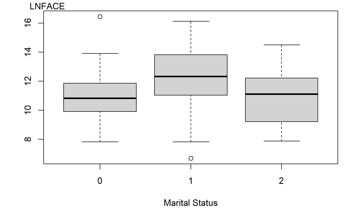
Figure 4.1: Box Plots of Logarithmic Face, by Level of Marital Status

R Code to Produce Table 4.1 and Figure 4.1

tableout <- 
  data.frame(
    MARSTAT <- c(0,1,2,""),
    Number <- c(57, 208, 10, 275),
    Mean <- c(10.958, 12.329, 10.825, 11.990),
    Standard_Deviation <- c(1.566, 1.822, 2.001, 1.871)
    )

colnames(tableout) <- c("MARSTAT", "Number", "Mean", "Standard Deviation")
rownames(tableout) <- c("Other", "Married", "Living together", "Total")

TableGen1(TableData=tableout , 
         TextTitle='Summary Statistics of Logarithmic Face By Marital Status', 
         Align='crrr', Digits=3, ColumnSpec=1:3,
         ColWidth = ColWidth4) %>%
         kableExtra::column_spec(1, width =  "4cm") 

library(HH)
Term   <- read.csv("CSVData/TermLife.csv", header=TRUE)
Term2  <- subset(Term, FACE > 0)
LNFACE <- log(Term2$FACE)
LNINCOME <- log(Term2$INCOME)
MAR0   <- 1*(Term2$MARSTAT == 0)

#  FIGURE 4.1
par(mar=c(4.1,4,1,1), cex=1.1)
boxplot(LNFACE ~ MARSTAT, data=Term2, ylab="",
   xlab="Marital Status")
mtext("LNFACE", side=2, at=17.2, las=1, cex=1.1, adj=.4)

Are the continuous and categorical variables jointly important determinants of response? To answer this, a regression was run using LNFACE as the response and five explanatory variables: three continuous and two binary (for marital status). Recall that our three continuous explanatory variables are: LNINCOME (logarithmic annual income), the number of years of EDUCATION of the survey respondent, and the number of household members, NUMHH.

For the binary variables, first define MAR0 to be the binary variable that is one if MARSTAT=0 and zero otherwise. Similarly, define MAR1 and MAR2 to be binary variables that indicate MARSTAT=1 and MARSTAT=2, respectively. There is a perfect linear dependency among these three binary variables in that MAR0 + MAR1 + MAR2 = 1 for any survey respondent. Thus, we need only two of the three. However, there is not a perfect dependency among any two of the three. It turns out that cor(MAR0, MAR1) = -0.90, cor(MAR0, MAR2) = -0.10, and cor(MAR1, MAR2) = -0.34.

A regression model was run using LNINCOME, EDUCATION, NUMHH, MAR0, and MAR2 as explanatory variables. The fitted regression equation turns out to be:

\[ \small{ \widehat{y} = 3.395 + 0.452 \text{ LNINCOME} + 0.205 \text{ EDUCATION} + 0.248 \text{ NUMHH} - 0.557 \text{ MAR0} - 0.789 \text{ MAR2}. } \]

To interpret the regression coefficients associated with marital status, consider a respondent who is married. In this case, MAR0=0, MAR1=1, and MAR2=0, so that:

\[ \small{ \widehat{y}_m = 3.395 + 0.452 \text{ LNINCOME} + 0.205 \text{ EDUCATION} + 0.248 \text{ NUMHH}. } \]

Similarly, if the respondent is coded as living together, then MAR0=0, MAR1=0, and MAR2=1, and:

\[ \small{ \widehat{y}_{lt} = 3.395 + 0.452 \text{ LNINCOME} + 0.205 \text{ EDUCATION} + 0.248 \text{ NUMHH} - 0.789. } \]

The difference between \(\widehat{y}_m\) and \(\widehat{y}_{lt}\) is \(0.789.\) Thus, we may interpret the regression coefficient associated with MAR2, \(-0.789\), to be the difference in fitted values for someone living together compared to a similar person who is married (the omitted category).

Similarly, we can interpret \(-0.557\) to be the difference between the “other” category and the married category, holding other explanatory variables fixed. For the difference in fitted values between the “other” and the “living together” categories, we may use \(-0.557 - (-0.789) = 0.232.\)

Although the regression was run using MAR0 and MAR2, any two out of the three would produce the same ANOVA Table (Table 4.2). However, the choice of binary variables does impact the regression coefficients. Table 4.3 shows three models, omitting MAR1, MAR2, and MAR0, respectively. For each fit, the coefficients associated with the continuous variables remain the same. As we have seen, the binary variable interpretations are with respect to the omitted category, known as the reference level. Although they change from model to model, their overall interpretation remains the same. That is, if we would like to estimate the difference in coverage between the “other” and the “living together” category, the estimate would be \(0.232\), regardless of the model.

Table 4.2: Term Life with Marital Status ANOVA Table

Source	Sum of Squares	\(df\)	Mean Square
Regression	343.28	5	68.66
Error	615.62	269	2.29
Total	948.90	274

Although the three models in Table 4.3 are the same except for different choices of parameters, they do appear different. In particular, the \(t\)-ratios differ and give different appearances of statistical significance. For example, both of the \(t\)-ratios associated with marital status in Model 2 are less than 2 in absolute value, suggesting that marital status is unimportant. In contrast, both Models 1 and 3 have at least one marital status binary that exceeds 2 in absolute value, suggesting statistical significance. Thus, you can influence the appearance of statistical significance by altering the choice of the reference level. To assess the overall importance of marital status (not just each binary variable), Section 4.2 will introduce tests of sets of regression coefficients.

Table 4.3: Term Life Regression Coefficients with Marital Status

	Model 1 Coefficient	Model 1 \(t\)-Ratio	Model 2 Coefficient	Model 2 \(t\)-Ratio	Model 3 Coefficient	Model 3 \(t\)-Ratio
LNINCOME	0.452	5.74	0.452	5.74	0.452	5.74
EDUCATION	0.205	5.3	0.205	5.3	0.205	5.3
NUMHH	0.248	3.57	0.248	3.57	0.248	3.57
Intercept	3.395	3.77	3.395	2.74	2.838	3.34
MAR0	-0.557	-2.15	0.232	0.44
MAR1			0.789	1.59	0.557	2.15
MAR2	-0.789	-1.59			-0.232	-0.44

---

Example: How does Cost-Sharing in Insurance Plans affect Expenditures in Healthcare? In one of many studies that resulted from the Rand Health Insurance Experiment (HIE) introduced in Section 1.5, Keeler and Rolph (1988) investigated the effects of cost-sharing in insurance plans. For this study, 14 health insurance plans were grouped by the co-insurance rate (the percentage paid as out-of-pocket expenditures that varied by 0, 25, 50 and 95%). One of the 95% plans limited annual out-of-pocket outpatient expenditures to 150 per person (450 per family), providing in effect an individual outpatient deductible. This plan was analyzed as a separate group so that there were \(c=5\) categories of insurance plans.

In most insurance studies, individuals choose insurance plans making it difficult to assess cost-sharing effects because of adverse selection. Adverse selection can arise because individuals in poor chronic health are more likely to choose plans with less cost sharing, thus giving the appearance that less coverage leads to greater expenditures. In the Rand HIE, individuals were randomly assigned to plans, thus removing this potential source of bias.

Keeler and Rolph (1988) organized an individual’s expenditures into episodes of treatment; each episode contains spending associated with a given bout of illness, chronic condition or procedure. Episodes were classified as hospital, dental or outpatient; this classification was based primarily on diagnoses, not by location of services. Thus, for example, outpatient services preceding or following a hospitalization, as well as related drugs and tests, were included as part of a hospital episode.

For simplicity, here we report only results for hospital episodes. Although families were randomly assigned to plans, Keeler and Rolph (1988) used regression methods to control for participant attributes and isolate the effects of plan cost-sharing. Table 4.4 summarizes the regression coefficients, based on a sample of \(n=1,967\) episode expenditures. In this regression, logarithmic expenditure was the dependent variable.

The cost-sharing categorical variable was decomposed into five binary variables so that no functional form was imposed on the response to insurance. These variables are “Co-ins25,” “Co-ins50,” and “Co-ins95,” for coinsurance rates 25, 50 and 95%, respectively, and “Indiv Deductible” for the plan with individual deductibles. The omitted variable is the free insurance plan with 0% coinsurance. The HIE was conducted in six cities; a categorical variable to control for the location was represented with five binary variables, Dayton, Fitchburg, Franklin, Charleston and Georgetown, with Seattle being the omitted variable. A categorical factor with \(c=6\) levels was used for age and sex; binary variables in the model consisted of “Age 0-2,” “Age 3-5,” “Age 6-17,” “Woman age 18-65,” and “Man age 46-65,” the omitted category was “Man age 18-45.” Other control variables included a health status scale, socioeconomic status, number of medical visits in the year prior to the experiment on a logarithmic scale and race.

Table 4.4 summarizes the effects of the variables. As noted by Keeler and Rolph, there were large differences by site and age although the regression only served to summarize \(R^2=11\%\) of the variability. For the cost-sharing variables, only “Co-ins95” was statistically significant, and this only at the 5% level, not the 1% level.

The paper of Keeler and Rolph (1988) examines other types of episode expenditures, as well as the frequency of expenditures. They concluded that cost-sharing of health insurance plans has little effect on the amount of expenditures per episode although there are important differences in the frequency of episodes. This is because an episode of treatment is composed of two decisions. The amount of treatment is made jointly between the patient and the physician and is largely unaffected by the type of health insurance plan. The decision to seek health care treatment is made by the patient; this decision-making process is more susceptible to economic incentives in cost-sharing aspects of health insurance plans.

Table 4.4: Coefficients of Episode Expenditures from the Rand HIE

Variable	Regression Coefficient	Variable	Regression Coefficient
Intercept	7.95
Dayton	0.13*	Co-ins25	0.07
Fitchburg	0.12	Co-ins50	0.02
Franklin	-0.01	Co-ins95	-0.13*
Charleston	0.20*	Indiv Deductible	-0.03
Georgetown	-0.18*
Health scale	-0.02*	Age 0-2	-0.63**
Socioeconomic status	0.03	Age 3-5	-0.64**
Medical visits	-0.03	Age 6-17	-0.30**
Examination	-0.10*	Woman age 18-65	0.11
Black	0.14*	Man age 46-65	0.26

Note: * significant at 5%, ** significant at 1%

Source: Keeler and Rolph (1988)

Video: Section Summary

4.2 Statistical Inference for Several Coefficients

It can be useful to examine several regression coefficients at the same time. For example, when assessing the effect of a categorical variable with \(c\) levels, we need to say something jointly about the \(c-1\) binary variables that enter the regression equation. To do this, Section 4.2.1 introduces a method for handling linear combinations of regression coefficients. Section 4.2.2 shows how to test several linear combinations, and Section 4.2.3 presents other inference applications.

4.2.1 Sets of Regression Coefficients

Recall that our regression coefficients are specified by \(\boldsymbol{\beta} = \left( \beta_0, \beta_1, \ldots, \beta_k \right)^{\prime},\) a \((k+1) \times 1\) vector. It will be convenient to express linear combinations of the regression coefficients using the notation \(\mathbf{C} \boldsymbol{\beta},\) where \(\mathbf{C}\) is a \(p \times (k+1)\) matrix that is user-specified and depends on the application. Some applications involve estimating \(\mathbf{C} \boldsymbol{\beta}\). Others involve testing whether \(\mathbf{C} \boldsymbol{\beta}\) equals a specific known value (denoted as \(\mathbf{d}\)). We call \(H_0:\mathbf{C \boldsymbol{\beta} = d}\) the general linear hypothesis. To demonstrate the broad variety of applications in which sets of regression coefficients can be used, we now present a series of special cases.

Special Case 1: One Regression Coefficient. In Section 3.4, we investigated the importance of a single coefficient, say \(\beta_j.\) We may express this coefficient as \(\mathbf{C} \boldsymbol{\beta}\) by choosing \(p=1\) and \(\mathbf{C}\) to be a \(1 \times (k+1)\) vector with a one in the \((j+1)\)st column and zeros otherwise. These choices result in

\[ \mathbf{C \boldsymbol{\beta} =} \left( 0~\ldots~0~1~0~\ldots~0\right) \left( \begin{array}{c} \beta_0 \\ \vdots \\ \beta_k \end{array} \right) = \beta_j. \]

Special Case 2: Regression Function. Here, we choose \(p=1\) and \(\mathbf{C}\) to be a \(1 \times (k+1)\) vector representing the transpose of a set of explanatory variables. These choices result in

\[ \mathbf{C \boldsymbol{\beta} =} \left( x_0, x_1, \ldots, x_k \right) \left( \begin{array}{c} \beta_0 \\ \vdots \\ \beta_k \end{array} \right) = \beta_0 x_0 + \beta_1 x_1 + \ldots + \beta_k x_k = \mathrm{E}~y, \] the regression function.

Special Case 3: Linear Combination of Regression Coefficients. When \(p=1\), we use the convention that lower-case bold letters are vectors and let \(\mathbf{C = c^{\prime}} = \left( c_0, \ldots, c_k \right)^{\prime}\). In this case, \(\mathbf{C} \boldsymbol{\beta}\) is a generic linear combination of regression coefficients

\[ \mathbf{C \boldsymbol{\beta} = \mathbf{c}^{\prime} \boldsymbol{\beta} = c_0 \beta_0 + \ldots + c_k \beta_k}. \]

Special Case 4: Testing Equality of Regression Coefficients. Suppose that the interest is in testing \(H_0: \beta_1 = \beta_2.\) For this purpose, let \(p=1\), \(\mathbf{c}^{\prime} = \left( 0, 1, -1, 0, \ldots, 0\right),\) and \(\mathbf{d} = 0\). With these choices, we have

\[ \mathbf{C \boldsymbol{\beta} = c^{\prime} \boldsymbol{\beta} =} \left( 0, 1, -1, 0, \ldots, 0\right) \left( \begin{array}{c} \beta_0 \\ \vdots \\ \beta_k \end{array} \right) = \beta_1 - \beta_2 = 0, \]

so that the general linear hypothesis reduces to \(H_0: \beta_1 = \beta_2.\)

Special Case 5: Adequacy of the Model. It is customary in regression analysis to present a test of whether or not any of the explanatory variables are useful for explaining the response. Formally, this is a test of the null hypothesis \(H_0:\beta_1=\beta_2=\ldots=\beta_k=0\). Note that, as a convention, one does not test whether or not the intercept is zero. To test this using the general linear hypothesis, we choose \(p=k\), \(\mathbf{d}=\left( 0~\ldots~0\right)^{\prime}\) to be a \(k \times 1\) vector of zeros and \(\mathbf{C}\) to be a \(k \times (k+1)\) matrix such that

\[ \small{ \mathbf{C \boldsymbol{\beta} =}\left( \begin{array}{ccccc} 0 & 1 & 0 & \cdots & 0 \\ 0 & 0 & 1 & \cdots & 0 \\ \vdots & \vdots & \vdots & \ddots & \vdots \\ 0 & 0 & 0 & \cdots & 1 \end{array} \right) \left( \begin{array}{c} \beta_0 \\ \vdots \\ \beta_k \end{array} \right) =\left( \begin{array}{c} \beta_1 \\ \vdots \\ \beta_k \end{array} \right) =\left( \begin{array}{c} 0 \\ \vdots \\ 0 \end{array} \right) =\mathbf{d}. } \]

Special Case 6: Testing Portions of the Model. Suppose that we are interested in comparing a full regression function

\[ \mathrm{E~}y = \beta_0 + \beta_1 x_1 +\ldots + \beta_k x_k + \beta_{k+1} x_{k+1} + \ldots + \beta_{k+p} x_{k+p} \] to a reduced regression function,

\[ \mathrm{E~}y = \beta_0 + \beta_1 x_1 + \ldots + \beta_k x_k. \] Beginning with the full regression, we see that if the null hypothesis \(H_0:\beta_{k+1} = \ldots = \beta_{k+p} = 0\) holds, then we arrive at the reduced regression. To illustrate, the variables \(x_{k+1}, \ldots, x_{k+p}\) may refer to several binary variables representing a categorical variable and our interest is in whether the categorical variable is important. To test the importance of the categorical variable, we want to see whether the binary variables \(x_{k+1}, \ldots, x_{k+p}\) jointly affect the dependent variables.

To test this using the general linear hypothesis, we choose \(\mathbf{d}\) and \(\mathbf{C}\) such that

\[ \small{ \mathbf{C \boldsymbol{\beta} =}\left( \begin{array}{ccccccc} 0 & \cdots & 0 & 1 & 0 & \cdots & 0 \\ 0 & \cdots & 0 & 0 & 1 & \cdots & 0 \\ \vdots & \vdots & \vdots & \vdots & \vdots & \ddots & \vdots \\ 0 & \cdots & 0 & 0 & 0 & \cdots & 1 \end{array} \right) \left( \begin{array}{c} \beta_0 \\ \vdots \\ \beta_k \\ \beta_{k+1} \\ \vdots \\ \beta_{k+p} \end{array} \right) =\left( \begin{array}{c} \beta_{k+1} \\ \vdots \\ \beta_{k+p} \end{array} \right) =\left( \begin{array}{c} 0 \\ \vdots \\ 0 \end{array} \right) =\mathbf{d}. } \]

From a list of \(k+p\) variables \(x_1, \ldots, x_{k+p}\), you may drop any \(p\) that you deem appropriate. The additional variables do not need to be the last \(p\) in the regression specification. Dropping \(x_{k+1}, \ldots, x_{k+p}\) is for notational convenience only.

Video: Summary

4.2.2 The General Linear Hypothesis

To recap, the general linear hypothesis can be stated as \(H_0:\mathbf{C \boldsymbol{\beta} =d}\). Here, \(\mathbf{C}\) is a \(p \times (k+1)\) matrix, \(\mathbf{d}\) is a \(p \times 1\) vector, and both \(\mathbf{C}\) and \(\mathbf{d}\) are user-specified and depend on the application at hand. Although \(k+1\) is the number of regression coefficients, \(p\) is the number of restrictions under \(H_0\) on these coefficients. (For those readers with knowledge of advanced matrix algebra, \(p\) is the rank of \(\mathbf{C}\).) This null hypothesis is tested against the alternative \(H_a:\mathbf{C \boldsymbol{\beta} \neq d}\). This may be obvious, but we do require \(p \leq k+1\) because we cannot test more constraints than free parameters.

To understand the basis for the testing procedure, we first recall some of the basic properties of the regression coefficient estimators described in Section 3.3. Now, however, our goal is to understand properties of the linear combinations of regression coefficients specified by \(\mathbf{C \boldsymbol{\beta}}\). A natural estimator of this quantity is \(\mathbf{Cb}\). It is easy to see that \(\mathbf{Cb}\) is an unbiased estimator of \(\mathbf{C \boldsymbol{\beta}}\), because \(\mathrm{E~}\mathbf{Cb=C}\mathrm{E~}\mathbf{b=C \boldsymbol{\beta}}\). Moreover, the variance is \(\mathrm{Var}\left( \mathbf{Cb}\right) \mathbf{=C}\mathrm{Var}\left( \mathbf{b}\right) \mathbf{C}^{\prime}=\sigma^2 \mathbf{C}\left( \mathbf{X^{\prime}X}\right)^{-1} \mathbf{C}^{\prime}\). To assess the difference between \(\mathbf{d}\), the hypothesized value of \(\mathbf{C \boldsymbol{\beta}}\), and its estimated value, \(\mathbf{Cb}\), we use the following statistic:

\[ F-\text{ratio}=\frac{(\mathbf{Cb-d)}^{\prime}\left( \mathbf{C}\left( \mathbf{X^{\prime}X} \right)^{-1} \mathbf{C}^{\prime}\right)^{-1}(\mathbf{Cb-d)}}{ps_{full}^2}. \tag{4.1} \]

Here, \(s_{full}^2\) is the mean square error from the full regression model. Using the theory of linear models, it can be checked that the statistic \(F\)-ratio has an \(F\)-distribution with numerator degrees of freedom \(df_1=p\) and denominator degrees of freedom \(df_2=n-(k+1)\). Both the statistic and the theoretical distribution are named for R. A. Fisher, a renowned scientist and statistician who did much to advance statistics as a science in the early half of the twentieth century.

Like the normal and the \(t\)-distribution, the \(F\)-distribution is a continuous distribution. The \(F\)-distribution is the sampling distribution for the \(F\)-ratio and is proportional to the ratio of two sums of squares, each of which is positive or zero. Thus, unlike the normal distribution and the \(t\)-distribution, the \(F\)-distribution takes on only nonnegative values. Recall that the \(t\)-distribution is indexed by a single degree of freedom parameter. The \(F\)-distribution is indexed by two degrees of freedom parameters: one for the numerator, \(df_1\), and one for the denominator, \(df_2\). Appendix A3.4 provides additional details.

The test statistic in equation (4.1) is complex in form. Fortunately, there is an alternative that is simpler to implement and to interpret; this alternative is based on the extra sum of squares principle.

Procedure for Testing the General Linear Hypothesis

1. Run the full regression and get the error sum of squares and mean square error, which we label as \((Error~SS)_{full}\) and \(s_{full}^2\), respectively.
2. Consider the model assuming the null hypothesis is true. Run a regression with this model and get the error sum of squares, which we label \((Error~SS)_{reduced}\).
3. Calculate \[ F-\text{ratio}=\frac{(Error~SS)_{reduced}-(Error~SS)_{full}}{ps_{full}^2}. \tag{4.2} \]
4. Reject the null hypothesis in favor of the alternative if the \(F\)-ratio exceeds an \(F\)-value. The \(F\)-value is a percentile from the \(F\)-distribution with \(df_1=p\) and \(df_2=n-(k+1)\) degrees of freedom. The percentile is one minus the significance level of the test. Following our notation with the \(t\)-distribution, we denote this percentile as \(F_{p,n-(k+1),1-\alpha}\), where \(\alpha\) is the significance level.

This procedure is commonly known as an \(F\)-test.

Section 4.7.2 provides the mathematical underpinnings. To understand the extra-sum-of-squares principle, recall that the error sum of squares for the full model is determined to be the minimum value of

\[ SS(b_0^{\ast}, \ldots, b_k^{\ast}) = \sum_{i=1}^{n} \left( y_i - \left( b_0^{\ast} + \ldots + b_k^{\ast} x_{i,k} \right) \right)^2. \]

Here, \(SS(b_0^{\ast}, \ldots, b_k^{\ast})\) is a function of \(b_0^{\ast}, \ldots, b_k^{\ast}\) and \((Error~SS)_{full}\) is the minimum over all possible values of \(b_0^{\ast}, \ldots, b_k^{\ast}\). Similarly, \((Error~SS)_{reduced}\) is the minimum error sum of squares under the constraints in the null hypothesis. Because there are fewer possibilities under the null hypothesis, we have that

\[ (Error~SS)_{full} \leq (Error~SS)_{reduced}. \tag{4.3} \]

To illustrate, consider our first special case where \(H_0 : \beta_j = 0\). In this case, the difference between the full and reduced models amounts to dropping a variable. A consequence of equation (4.3) is that, when adding variables to a regression model, the error sum of squares never goes up (and, in fact, usually goes down). Thus, adding variables to a regression model increases \(R^2\), the coefficient of determination.

How large a decrease in the error sum of squares is statistically significant? Intuitively, one can view the \(F\)-ratio as the difference in the error sum of squares divided by the number of constraints, \(\frac{(Error~SS)_{reduced}-(Error~SS)_{full}}{p}\), and then rescaled by the best estimate of the variance term, the \(s^2\), from the full model. Under the null hypothesis, this statistic follows an \(F\)-distribution and we may compare the test statistic to this distribution to see if it is unusually large.

Using the relationship \(Regression~SS = Total~SS - Error~SS\), we can re-express the difference in the error sum of squares as

\[ (Error~SS)_{reduced} - (Error~SS)_{full} = (Regression~SS)_{full} - (Regression~SS)_{reduced}. \]

This difference is known as a Type III Sum of Squares. When testing the importance of a set of explanatory variables, \(x_{k+1}, \ldots, x_{k+p}\), in the presence of \(x_1, \ldots, x_k\), you will find that many statistical software packages compute this quantity directly in a single regression run. The advantage of this is it allows the analyst to perform an \(F\)-test using a single regression run, instead of two regression runs as in our four-step procedure described above.

---

Example: Term Life Insurance - Continued. Before discussing the logic and the implications of the \(F\)-test, let us illustrate its use. In the Term Life Insurance example, suppose that we wish to understand the impact of marital status. Table 4.3 presented a mixed message in terms of \(t\)-ratios; sometimes they were statistically significant and sometimes not. It would be helpful to have a formal test to give a definitive answer, at least in terms of statistical significance. Specifically, we consider a regression model using LNINCOME, EDUCATION, NUMHH, MAR0, and MAR2 as explanatory variables. The model equation is

\[ \small{ \begin{array}{ll} y &= \beta_0 + \beta_1 \text{LNINCOME} + \beta_2 \text{EDUCATION} + \beta_3 \text{NUMHH} \\ & \ \ \ \ + \beta_4 \text{MAR0} + \beta_5 \text{MAR2}. \end{array} } \]

Our goal is to test \(H_0: \beta_4 = \beta_5 = 0\).

1. We begin by running a regression model with all \(k+p=5\) variables. The results were reported in Table 4.2, where we saw that \((Error~SS)_{full} = 615.62\) and \(s_{full}^2 = (1.513)^2 = 2.289\).
2. The next step is to run the reduced model without MAR0 and MAR2. This was done in Table 3.3 of Chapter 3, where we saw that \((Error~SS)_{reduced} = 630.43\).
3. We then calculate the test statistic \[ F-\text{ratio} = \frac{(Error~SS)_{reduced} - (Error~SS)_{full}}{ps_{full}^2} = \frac{630.43 - 615.62}{2 \times 2.289} = 3.235. \]
4. The fourth step compares the test statistic to an \(F\)-distribution with \(df_1=p=2\) and \(df_2 = n-(k+p+1) = 269\) degrees of freedom. Using a 5% level of significance, it turns out that the 95th percentile is \(F-\text{value} \approx 3.029\). The corresponding \(p\)-value is \(\Pr(F > 3.235) = 0.0409\). At the 5% significance level, we reject the null hypothesis \(H_0: \beta_4 = \beta_5 = 0\). This suggests that it is important to use marital status to understand term life insurance coverage, even in the presence of income, education, and number of household members.

---

Some Special Cases

The general linear hypothesis test is available when you can express one model as a subset of another. For this reason, it is useful to think of it as a device for comparing “smaller” to “larger” models. However, the smaller model must be a subset of the larger model. For example, the general linear hypothesis test cannot be used to compare the regression functions \(\mathrm{E~}y = \beta_0 + \beta_7 x_7\) versus \(\mathrm{E~}y = \beta_0 + \beta_1 x_1 + \beta_2 x_2 + \beta_3 x_3 + \beta_4 x_4\). This is because the former, smaller function is not a subset of the latter, larger function.

The general linear hypothesis can be used in many instances, although its use is not always necessary. For example, suppose that we wish to test \(H_0:\beta_k=0\). We have already seen that this null hypothesis can be examined using the \(t\)-ratio test. In this special case, it turns out that \((t-\textrm{ratio})^2=F-\textrm{ratio}\). Thus, these tests are equivalent for testing \(H_0:\beta_k=0\) versus \(H_a:\beta_k \neq 0\). The \(F\)-test has the advantage that it works for more than one predictor whereas the \(t\)-test has the advantage that one can consider one-sided alternatives. Thus, both tests are considered useful.

Dividing the numerator and denominator of equation (4.4) by \(Total~SS\), the test statistic can also be written as:

\[ F-\textrm{ratio}=\frac{\left( R_{full}^2-R_{reduced}^2\right) /p}{\left( 1-R_{full}^2\right) / (n-(k+1))}. \tag{4.4} \]

The interpretation of this expression is that the \(F\)-ratio measures the drop in the coefficient of determination, \(R^2\).

The expression in equation (4.4) is particularly useful for testing the adequacy of the model, our Special Case 5. In this case, \(p=k\), and the regression sum of squares under the reduced model is zero. Thus, we have

\[ \small{ F-\textrm{ratio}=\frac{\left( (Regression~SS)_{full}\right) /k}{s_{full}^2} =\frac{(Regression~MS)_{full}}{(Error~SS)_{full}}. } \]

This test statistic is a regular feature of the ANOVA table for many statistical packages.

For example, in our Term Life Insurance example, testing the adequacy of the model means evaluating \(H_0: \beta_1 = \beta_2 =\beta_3 =\beta_4 =\beta_5 = 0\). From Table 4.2, the \(F\)-ratio is 68.66 / 2.29 = 29.98. With \(df_1=5\) and \(df_2 = 269\), we have that the \(F\)-value is approximately 2.248 and the corresponding \(p\)-value is \(\Pr(F > 29.98) \approx 0\). This leads us to reject strongly the notion that the explanatory variables are not useful in understanding term life insurance coverage, reaffirming what we learned in the graphical and correlation analysis. Any other result would be surprising.

For another expression, dividing by \(Total~SS\), we may write

\[ F-\textrm{ratio}=\frac{R^2}{1-R^2}\frac{n-(k+1)}{k}. \]

Because both \(F\)-ratio and \(R^2\) are measures of model fit, it seems intuitively plausible that they be related in some fashion. A consequence of this relationship is the fact that as \(R^2\) increases, so does the \(F\)-ratio and vice versa. The \(F\)-ratio is used because its sampling distribution is known under a null hypothesis so we can make statements about statistical significance. The \(R^2\) measure is used because of the easy interpretations associated with it.

Video: Summary

4.2.3 Estimating and Predicting Several Coefficients

Estimating Linear Combinations of Regression Coefficients

In some applications, the main interest is to estimate a linear combination of regression coefficients. To illustrate, recall in Section 3.5 that we developed a regression function for an individual’s charitable contributions (\(y\)) in terms of their wages (\(x\)). In this function, there was an abrupt change in the function at \(x=97,500\). To model this, we defined the binary variable \(z\) to be zero if \(x<97,500\) and to be one if \(x \geq 97,500\), and the regression function \(\mathrm{E~}y = \beta_0 + \beta_1 x + \beta_2 z(x - 97,500)\). Thus, the marginal expected change in contributions per dollar wage change for wages in excess of \(97,500\) is \(\frac{\partial \left( \mathrm{E~}y\right)}{\partial x} = \beta_1 + \beta_2\).

To estimate \(\beta_1 + \beta_2\), a reasonable estimator is \(b_1 + b_2\) which is readily available from standard regression software. In addition, we would also like to compute standard errors for \(b_1 + b_2\) to be used, for example, in determining a confidence interval for \(\beta_1 + \beta_2\). However, \(b_1\) and \(b_2\) are typically correlated so that the calculation of the standard error of \(b_1 + b_2\) requires estimation of the covariance between \(b_1\) and \(b_2\).

Estimating \(\beta_1 + \beta_2\) is an example of our Special Case 3 that considers linear combinations of regression coefficients of the form \(\mathbf{c}^{\prime} \boldsymbol \beta = c_0 \beta_0 + c_1 \beta_1 + \ldots + c_k \beta_k\). For our charitable contribution’s example, we would choose \(c_1 = c_2 = 1\) and other \(c\)’s equal to zero.

To estimate \(\mathbf{c}^{\prime} \boldsymbol \beta\), we replace the vector of parameters by the vector of estimators and use \(\mathbf{c}^{\prime} \mathbf{b}\). To assess the reliability of this estimator, as in Section 4.2.2, we have that \(\mathrm{Var}\left( \mathbf{c}^{\prime} \mathbf{b}\right) = \sigma^2 \mathbf{c}^{\prime}(\mathbf{X^{\prime} X})^{-1} \mathbf{c}\). Thus, we may define the estimated standard deviation, or standard error, of \(\mathbf{c}^{\prime} \mathbf{b}\) to be

\[ se\left( \mathbf{c}^{\prime} \mathbf{b} \right) = s \sqrt{\mathbf{c}^{\prime} (\mathbf{X}^{\prime} \mathbf{X})^{-1} \mathbf{c}}. \]

With this quantity, a \(100(1 - \alpha) \%\) confidence interval for \(\mathbf{c}^{\prime} \boldsymbol \beta\) is

\[ \mathbf{c}^{\prime} \mathbf{b} \pm t_{n - (k + 1), 1 - \alpha / 2} ~ se(\mathbf{c}^{\prime} \mathbf{b}). \tag{4.5} \]

The confidence interval in equation (4.5) is valid under Assumptions F1-F5. If we choose \(\mathbf{c}\) to have a “1” in the \((j + 1)^{\text{st}}\) row and zeros otherwise, then \(\mathbf{c}^{\prime} \boldsymbol \beta = \beta_j\), \(\mathbf{c}^{\prime} \mathbf{b} = b_j\), and

\[ se(b_j) = s \sqrt{(j + 1)^{\text{st}}~ \textit{diagonal element of } (\mathbf{X}^{\prime} \mathbf{X})^{-1}}. \]

Thus, equation (4.5) provides a theoretical basis for the individual regression coefficient confidence intervals introduced in Section 3.4’s equation (3.10) and generalizes it to arbitrary linear combinations of regression coefficients.

Another important application of equation (4.5) is the choice of \(\mathbf{c}\) corresponding to a set of explanatory variables of interest, say, \(\mathbf{x}_{\ast} = \left( 1, x_{\ast 1}, x_{\ast 2}, \ldots, x_{\ast k} \right)^{\prime}\). These may correspond to an observation within the data set or to a point outside the available data. The parameter of interest, \(\mathbf{c}^{\prime} \boldsymbol \beta = \mathbf{x}_{\ast}^{\prime} \boldsymbol \beta\), is the expected response or the regression function at that point. Then, \(\mathbf{x}_{\ast}^{\prime} \mathbf{b}\) provides a point estimator and equation (4.5) provides the corresponding confidence interval.

Prediction Intervals

Prediction is an inferential goal that is closely related to estimating the regression function at a point. Suppose that, when considering charitable contributions, we know an individual’s wages (and thus whether wages are in excess of \(97,500\)) and wish to predict the amount of charitable contributions. In general, we assume that the set of explanatory variables \(\mathbf{x}_{\ast}\) is known and wish to predict the corresponding response \(y_{\ast}\). This new response follows the assumptions as described in Section 3.2. Specifically, the expected response is \(\mathrm{E~}y_{\ast} = \mathbf{x}_{\ast}^{\prime} \boldsymbol \beta\), \(\mathbf{x}_{\ast}\) is nonstochastic, \(\mathrm{Var~}y_{\ast} = \sigma^2\), \(y_{\ast}\) is independent of \(\{y_1, \ldots, y_{n}\}\) and is normally distributed. Under these assumptions, a \(100(1 - \alpha)\%\) prediction interval for \(y_{\ast}\) is

\[ \mathbf{x}_{\ast}^{\prime} \mathbf{b} \pm t_{n - (k + 1), 1 - \alpha / 2} ~ s \sqrt{1 + \mathbf{x}_{\ast}^{\prime} (\mathbf{X}^{\prime} \mathbf{X})^{-1} \mathbf{x}_{\ast}}. \tag{4.6} \]

Equation (4.6) generalizes the prediction interval introduced in Section 2.4.

Video: Summary

4.3 One Factor ANOVA Model

Section 4.1 showed how to incorporate unordered categorical variables, or factors, into a linear regression model through the use of binary variables. Factors are important in social science research; they can be used to classify people by gender, ethnicity, marital status and so on, or classify firms by geographic region, organizational structure and so forth. Within studies of insurance, factors are used by insurers to categorize policyholders according to a “risk classification system.” Here, the idea is to create groups of policyholders with similar risk characteristics that will have similar claims experience. These groups form the basis of insurance pricing, so that each policyholder is charged an amount that is appropriate to their risk category. This process is sometimes known as “segmentation.”

Although factors may be represented as binary variables in a linear regression model, we study one factor models as a separate unit because:

• The method of least squares is much simpler, obviating the need to take inverses of high-dimensional matrices.
• The resulting interpretations of coefficients are more straightforward.

The one factor model is still a special case of the linear regression model. Hence, no additional statistical theory is needed to establish its statistical inference capabilities.

To establish notation for the one factor ANOVA model, we now consider the following example.

---

Example: Automobile Insurance Claims. We examine claims experience from a large midwestern (US) property and casualty insurer for private passenger automobile insurance. The dependent variable is the amount paid on a closed claim, in (US) dollars (claims that were not closed by year end are handled separately). Insurers categorize policyholders according to a risk classification system. This insurer’s risk classification system is based on:

• Automobile operator characteristics (age, gender, marital status and whether the primary or occasional driver of a car).
• Vehicle characteristics (city versus farm usage, if the vehicle is used to commute to school or work, used for business or pleasure, and if commuting, the approximate distance of the commute).

These factors are summarized by the risk class categorical variable CLASS. Table 4.5 shows 18 risk classes - further classification information is not given here to protect proprietary interests of the insurer.

Table 4.5 summarizes the results from \(n=6,773\) claims for drivers aged 50 and above. We can see that the median claim varies from a low of $707.40 (CLASS F7) to a high of 1,231.25 (CLASS C72). The distribution of claims turns out to be skewed, so we consider \(y\) = logarithmic claims. The table presents means, medians and standard deviations. Because the distribution of logarithmic claims is less skewed, means are close to medians. Figure 4.2 shows the distribution of logarithmic claims by risk class.

Table 4.5: Automobile Claims Summary Statistics by Risk Class

	1	2	3	4	5	6
Class	C1	C11	C1A	C1B	C1C	C2
Number	726	1151	77	424	38	61
Median (dollars)	948.86	1,013.81	925.48	1,026.73	1,001.73	851.20
Median (in log dollars)	6.855	6.921	6.830	6.934	6.909	6.747
Mean (in log dollars)	6.941	6.952	6.866	6.998	6.786	6.801
Std. dev. (in log dollars)	1.064	1.074	1.072	1.068	1.110	0.948
Class	C6	C7	C71	C72	C7A	C7B
Number	911	913	1129	85	113	686
Median (dollars)	1,011.24	957.68	960.40	1,231.25	1,139.93	1,113.13
Median (in log dollars)	6.919	6.865	6.867	7.116	7.039	7.015
Mean (in log dollars)	6.926	6.901	6.954	7.183	7.064	7.072
Std. dev. (in log dollars)	1.115	1.058	1.038	0.988	1.021	1.103
Class	C7C	F1	F11	F6	F7	F71
Number	81	29	40	157	59	93
Median (dollars)	1,200.00	1,078.04	774.79	1,105.04	707.40	1,118.73
Median (in log dollars)	7.090	6.983	6.652	7.008	6.562	7.020
Mean (in log dollars)	7.244	7.004	6.804	6.910	6.577	6.935
Std. dev. (in log dollars)	0.944	0.996	1.212	1.193	0.897	0.983

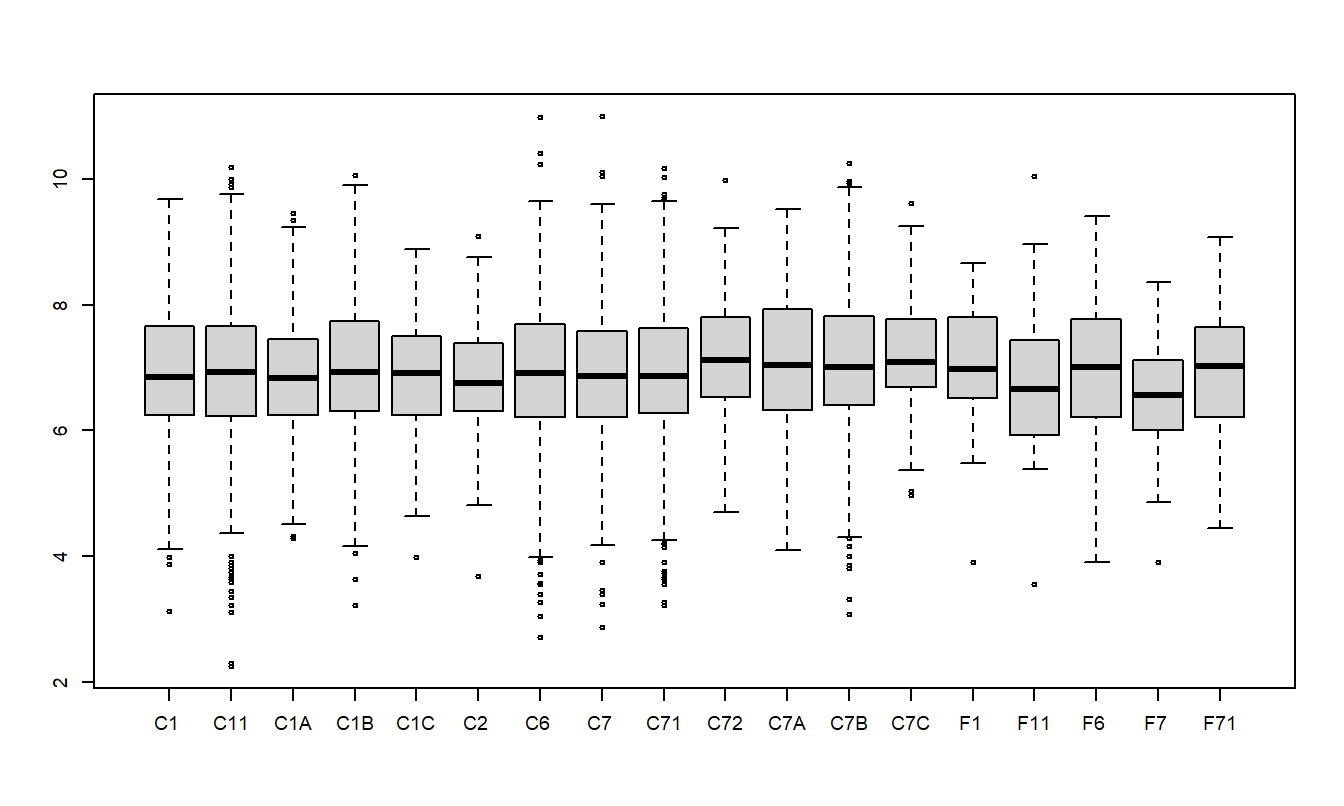
Figure 4.2: Box Plots of Logarithmic Claims by Risk Class

R Code to Produce Table 4.5 and Figure 4.2

AutoC   <- read.csv("CSVData/AutoClaims.csv", header=TRUE)
#  CREATE A TABLE OF MEANS AND STANDARD DEVIATIONS
library(Hmisc)
t1 <- summarize(log(AutoC$PAID), AutoC$CLASS, length ) 
t2 <- summarize(AutoC$PAID, AutoC$CLASS, median) 
t3 <- summarize(log(AutoC$PAID), AutoC$CLASS, median) 
t4 <- summarize(log(AutoC$PAID), AutoC$CLASS, mean) 
t5 <- summarize(log(AutoC$PAID), AutoC$CLASS, sd) 
tablemat <- cbind(t1,
                  format(round(t2[2], digits = 2), big.mark = ','),
                  round(t3[2], digits = 3),
                  round(t4[2], digits = 3),
                  round(t5[2], digits = 3))
block1 <-  t(tablemat[1:6,])
block2 <- t(tablemat[7:12,])
block3 <- t(tablemat[13:18,])

#tableout[3,] <- format(round(tableout[3,], digits=0), big.mark = ',')

bigblock <- rbind(block1, block2, block3)
temprow <- c("Class", "Number", "Median (dollars)", "Median (in log dollars)" ,"Mean (in log dollars)", "Std. dev. (in log dollars)") 
bigblock1 <- cbind (c(temprow,temprow, temprow), bigblock)
row.names(bigblock1) <- NULL

TableGen1(TableData=bigblock1 , 
         TextTitle='Automobile Claims Summary Statistics by Risk Class', 
         Align='lrrrrrr', Digits=3, ColumnSpec=1:6,
         ColWidth = ColWidth4) %>%
       kableExtra::column_spec(1, width =  "4cm") %>%
     kableExtra::row_spec(6, extra_css = "border-bottom: 2px solid black;") %>%
     kableExtra::row_spec(12, extra_css = "border-bottom: 2px solid black;")

library(HH)
AutoC   <- read.csv("CSVData/AutoClaims.csv", header=TRUE)
#  AUTO CLAIMS
#  FIGURE 4.2

par(cex=0.6)
boxplot(log(PAID) ~ CLASS,cex=.6, cex.labels=2, data = AutoC,
        xlab = "", ylab = "")

---

This section focuses on the risk class (CLASS) as the explanatory variable. We use the notation \(y_{ij}\) to mean the \(i\)th observation of the \(j\)th risk class. For the \(j\)th risk class, we assume there are \(n_j\) observations. There are \(n=n_1+n_2+\ldots +n_c\) observations. The data are:

\[ \begin{array}{cccccc} \text{Data for risk class }1 & \ \ \ \ & y_{11} & y_{21} & \ldots & y_{n_1,1} \\ \text{Data for risk class }2 & & y_{12} & y_{22} & \ldots & y_{n_2,1} \\ . & & . & . & \ldots & . \\ \text{Data for risk class } c & & y_{1c} & y_{2c} & \ldots & y_{n_c,c} \end{array} \]

where \(c=18\) is the number of levels of the CLASS factor. Because each level of a factor can be arranged in a single row (or column), another term for this type of data is a “one way classification.” Thus, a one way model is another term for a one factor model.

An important summary measure of each level of the factor is the sample average. Let \[ \overline{y}_j=\frac{1}{n_j}\sum_{i=1}^{n_j}y_{ij} \] denote the average from the \(j\)th CLASS.

Model Assumptions and Analysis

The one factor ANOVA model equation is \[ y_{ij}=\mu_j+ \varepsilon_{ij}\ \ \ \ \ \ i=1,\ldots ,n_j,\ \ \ \ \ j=1,\ldots ,c. \tag{4.7} \] As with regression models, the random deviations \(\{\varepsilon_{ij} \}\) are assumed to be zero mean with constant variance (Assumption E3) and independent of one another (Assumption E4). Because we assume the expected value of each deviation is zero, we have \(\text{E}~y_{ij}=\mu_j\). Thus, we interpret \(\mu_j\) to be the expected value of the response \(y_{ij}\), that is, the mean \(\mu\) varies by the \(j\)th factor level.

To estimate the parameters \(\{\mu_j\}\), as with regression we use the method of least squares, introduced in Section 2.1. That is, let \(\mu^{\ast}_j\) be a “candidate” estimate of \(\mu_j\). The quantity \[ SS(\mu^{\ast}_1, \ldots , \mu^{\ast}_{c}) = \sum_{j=1}^{c} \sum_{i=1}^{n_j} (y_{ij}-\mu^{\ast}_j)^2 \] represents the sum of squared deviations of the responses from these candidate estimates. From straightforward algebra, the value of \(\mu^{\ast}_j\) that minimizes this sum of squares is \(\bar{y}_j\). Thus, \(\bar{y}_j\) is the least squares estimate of \(\mu_j\).

To understand the reliability of the estimates, we can partition the variability as in the regression case, presented in Sections 2.3.1 and 3.3. The minimum sum of squared deviations is called the error sum of squares and is defined to be \[ Error ~SS = SS(\bar{y}_1, \ldots, \bar{y}_{c}) = \sum_{j=1}^{c} \sum_{i=1}^{n_j} \left(y_{ij}-\bar{y}_j \right)^2. \] The total variation in the data set is summarized by the total sum of squares, \[ Total ~SS=\sum_{j=1}^{c}\sum_{i=1}^{n_j}(y_{ij}-\bar{y})^2. \] The difference, called the factor sum of squares, can be expressed as: \[ \begin{array}{ll} Factor~ SS & = Total ~SS - Error ~SS \\ & = \sum_{j=1}^{c}\sum_{i=1}^{n_j}(y_{ij}-\bar{y})^2-\sum_{j=1}^{c}\sum_{i=1}^{n_j}(y_{ij}-\bar{y}_j)^2 = \sum_{j=1}^{c}\sum_{i=1}^{n_j}(\bar{y}_j-\bar{y})^2 \\ & = \sum_{j=1}^{c}n_j(\bar{y}_j-\bar{y})^2. \end{array} \] The last two equalities follow from algebra manipulation. The \(Factor ~SS\) plays the same role as the \(Regression ~SS\) in Chapters 2 and 3. The variability decomposition is summarized in Table 4.6.

Table 4.6: ANOVA Table for One Factor Model

Source	Sum of Squares	\(df\)	Mean Square
Factor	\(Factor ~SS\)	\(c-1\)	\(Factor ~MS\)
Error	\(Error ~SS\)	\(n-c\)	\(Error ~MS\)
Total	\(Total ~SS\)	\(n-1\)

The conventions for this table are the same as in the regression case. That is, the mean square (MS) column is defined by the sum of squares (SS) column divided by the degrees of freedom (df) column. Thus, \(Factor~MS \equiv (Factor~SS)/(c-1)\) and \(Error~MS \equiv (Error~SS)/(n-c)\). We use \[ s^2 = \text{Error MS} = \frac{1}{n-c} \sum_{j=1}^{c}\sum_{i=1}^{n_j} e_{ij}^2 \] to be our estimate of \(\sigma^2\), where \(e_{ij} = y_{ij} - \bar{y}_j\) is the residual.

With this value for \(s\), it can be shown that the interval estimate for \(\mu_j\) is \[ \bar{y}_j \pm t_{n-c,1-\alpha /2}\frac{s}{\sqrt{n_j}}. \tag{4.8} \]

Here, the t-value \(t_{n-c,1-\alpha /2}\) is a percentile from the t-distribution with \(df=n-c\) degrees of freedom.

---

Example: Automobile Claims - Continued. To illustrate, the ANOVA table summarizing the fit for the automobile claims data appears in Table 4.7. Here, we see that the mean square error is \(s^2 = 1.14.\)

Table 4.7: ANOVA Table for Logarithmic Automobile Claims

Source	Sum of Squares	\(df\)	Mean Square
CLASS	39.2	17	2.31
Error	7729.0	6755	1.14
Total	7768.2	6772

In automobile ratemaking, one uses the average claims to help set prices for insurance coverages. As an example, for CLASS C72 the average logarithmic claim is 7.183. From equation (4.8), a 95% confidence interval is \[ 7.183 \pm (1.96) \frac{\sqrt{1.14}}{\sqrt{85}} = 7.183 \pm 0.227 = (6.956 ,7.410). \] Note that these estimates are in natural logarithmic units. In dollars, our point estimate is \(e^{7.183} = 1,316.85\) and our 95% confidence interval is \((e^{6.956} , e^{7.410}) \text{ or } (\$1,049.43, \$1,652.43)\).

---

An important feature of the one factor ANOVA decomposition and estimation is the ease of computation. Although the sum of squares appear complex, it is important to note that no matrix calculations are required. Rather, all of the calculations can be done through averages and sums of squares. This has been an important consideration historically, before the age of readily available desktop computing. Moreover, insurers may segment their portfolios into hundreds or even thousands of risk classes instead of the 18 used in our Automobile Claims data. Thus, even today it can be helpful to identify a categorical variable as a factor and let your statistical software use ANOVA estimation techniques. Further, ANOVA estimation also provides for direct interpretation of the results.

Link with Regression

This subsection shows how a one factor ANOVA model can be rewritten as a regression model. To this end, we have seen that both the regression model and one factor ANOVA model use a linear error structure with Assumptions E3 and E4 for identically and independently distributed errors. Similarly, both use the normality assumption E5 for selected inference results (such as confidence intervals). Both employ non-stochastic explanatory variables as in Assumption E2. Both have an additive (mean zero) error term, so the main apparent difference is in the expected response, \(\mathrm{E }~y\).

For the linear regression model, \(\mathrm{E }~y\) is a linear combination of explanatory variables (Assumption F1). For the one factor ANOVA model, \(E[y_j] = \mu_j\) is a mean that depends on the level of the factor. To equate these two approaches, for the ANOVA factor with \(c\) levels, we define \(c\) binary variables, \(x_1, x_2, \ldots, x_c\). Here, \(x_j\) indicates whether or not an observation falls in the \(j\)th level. With these variables, we can rewrite our one factor ANOVA model as \[ y = \mu_1 x_1 + \mu_2 x_2 + \ldots + \mu_c x_c + \varepsilon. \tag{4.9} \] Thus, we have re-written the one factor ANOVA expected response as a regression function, although using a no-intercept form (as in equation (3.5)).

The one factor ANOVA is a special case of our usual regression model, using binary variables from the factor as explanatory variables in the regression function. As we have seen, no matrix calculations are needed for least squares estimation. However, one can always use the matrix procedures developed in Chapter 3. Section 4.7.1 shows how our usual matrix expression for regression coefficients (\(\mathbf{b} = \left(\mathbf{X}^{\prime}\mathbf{X}\right)^{-1}\mathbf{X}^{\prime}\mathbf{y}\)) reduces to the simple estimates \(\bar{y}_j\) when using only one categorical variable.

Reparameterization

To include an intercept term, define \(\tau_j = \mu_j - \mu\), where \(\mu\) is an, as yet, unspecified parameter. Because each observation must fall into one of the \(c\) categories, we have \(x_1 + x_2 + \ldots + x_{c} = 1\) for each observation. Thus, using \(\mu_j = \tau_j + \mu\) in equation (4.9), we have \[ y = \mu + \tau_1 x_1 + \tau_2 x_2 + \ldots + \tau_{c} x_{c} + \varepsilon, \tag{4.10} \] we have re-written the model into what appears to be our usual regression format.

We use the \(\tau\) in lieu of \(\beta\) for historical reasons. ANOVA models were invented by R.A. Fisher in connection with agricultural experiments. Here, the typical set-up is to apply several treatments to plots of land in order to quantify crop yield responses. Thus, the Greek “t”, \(\tau\), suggests the word treatment, another term used to describe levels of the factor of interest.

A simpler version of equation (4.10) \[ y_{ij} = \mu + \tau_j + \varepsilon_{ij}. \] can be given when we identify the factor level. That is, if we know an observation falls in the \(j\)th level, then only \(x_j\) is one and the other \(x\)’s are 0. Thus, a simpler expression for equation (4.10) \[ y_{ij} = \mu + \tau_j + \varepsilon_{ij}. \]

Comparing equations (4.9) and (4.10), we see that the number of parameters has increased by one. That is, in equation (4.9) there are \(c\) parameters, \(\mu_1, \ldots, \mu_c\), even though in equation (4.10) there are \(c + 1\) parameters, \(\mu\) and \(\tau_1, \ldots, \tau_c\). The model in equation (4.10) is said to be overparameterized. It is possible to estimate this model directly, using the general theory of linear models, summarized in Section 4.7.3. In this theory, regression coefficients need not be identifiable. Alternatively, one can make these two expressions equivalent by restricting the movement of the parameters in equation (4.10). We now present two ways of imposing restrictions.

The first type of restriction, usually done in the regression context, is to require one of the \(\tau\)’s to be zero. This amounts to dropping one of the explanatory variables. For example, we might use \[ y = \mu + \tau_1 x_1 + \tau_2 x_2 + \ldots + \tau_{c-1} x_{c-1} + \varepsilon, \tag{4.11} \] dropping \(x_c\). With this formulation, it is easy to fit the model in equation (4.11) using regression statistical software routines because one only needs to run the regression with \(c-1\) explanatory variables. However, one needs to be careful with the interpretation of parameters. To equate the models in equations (4.9) and (4.10), we need to define \(\mu \equiv \mu_c\) and \(\tau_j = \mu_j - \mu_c\) for \(j=1,2,\ldots,c-1\). That is, the regression intercept term is the mean level of the category dropped, and each regression coefficient is the difference between a mean level and the mean level dropped. It is not necessary to drop the last level \(c\), and indeed, one could drop any level. However, the interpretation of the parameters does depend on the variable dropped. With this restriction, the fitted values are \(\hat{\mu} = \hat{\mu}_c = \bar{y}_c\) and \(\hat{\tau}_j = \hat{\mu}_j - \hat{\mu}_c = \bar{y}_j - \bar{y}_c.\) Recall that the caret (\(\hat{\cdot}\)), or “hat,” stands for an estimated, or fitted, value.

The second type of restriction is to interpret \(\mu\) as a mean for the entire population. To this end, the usual requirement is \(\mu \equiv \frac{1}{n} \sum_{j=1}^c n_j \mu_j,\) that is, \(\mu\) is a weighted average of means. With this definition, we interpret \(\tau_j = \mu_j - \mu\) as treatment differences between a mean level and the population mean. Another way of expressing this restriction is \(\sum_{j=1}^{c} n_j \tau_j = 0,\) that is, the (weighted) sum of treatment differences is zero. The disadvantage of this restriction is that it is not readily implementable with a regression routine and a special routine is needed. The advantage is that there is a symmetry in the definitions of the parameters. There is no need to worry about which variable is being dropped from the equation, an important consideration. With this restriction, the fitted values are \[ \hat{\mu} = \frac{1}{n} \sum_{j=1}^{c} n_j \hat{\mu}_j = \frac{1}{n} \sum_{j=1}^{c} n_j \bar{y}_j = \bar{y} \] and \[ \hat{\tau}_j = \hat{\mu}_j - \hat{\mu} = \bar{y}_j - \bar{y}. \]

Video: Section Summary

4.4 Combining Categorical and Continuous Explanatory Variables

There are several ways to combine categorical and continuous explanatory variables. We initially present the case of only one categorical and one continuous variable. We then briefly present the general case, called the general linear model. When combining categorical and continuous variable models, we use the terminology factor for the categorical variable and covariate for the continuous variable.

Combining a Factor and Covariate

Let us begin with the simplest models that use a factor and a covariate. In Section 4.3, we introduced the one factor model \(y_{ij} = \mu_j + \varepsilon_{ij}\). In Chapter 2, we introduced basic linear regression in terms of one continuous variable, or covariate, using \(y_{ij} = \beta_0 + \beta_1 x_{ij} + \varepsilon_{ij}\). Table 4.8 summarizes different approaches that could be used to represent combinations of a factor and covariate.

Table 4.8: Several Models that Represent Combinations of One Factor and One Covariate

Model Description	Notation
One factor ANOVA (no covariate model)	\(y_{ij} = \mu_j + \varepsilon_{ij}\)
Regression with constant intercept and slope (no factor model)	\(y_{ij} = \beta_0 + \beta_1 x_{ij} + \varepsilon_{ij}\)
Regression with variable intercept and constant slope (analysis of covariance model)	\(y_{ij} = \beta_{0j} + \beta_1 x_{ij} + \varepsilon_{ij}\)
Regression with constant intercept and variable slope	\(y_{ij} = \beta_0 + \beta_{1j} x_{ij} + \varepsilon_{ij}\)
Regression with variable intercept and slope	\(y_{ij} = \beta_{0j} + \beta_{1j} x_{ij} + \varepsilon_{ij}\)

We can interpret the regression with variable intercept and constant slope to be an additive model, because we are adding the factor effect, \(\beta_{0j}\), to the covariate effect, \(\beta_1 x_{ij}\). Note that one could also use the notation, \(\mu_j\), in lieu of \(\beta_{0j}\) to suggest the presence of a factor effect. This is also known as an analysis of covariance (ANCOVA) model. The regression with variable intercept and slope can be thought of as an interaction model. Here, both the intercept, \(\beta_{0j}\), and slope, \(\beta_{1j}\), may vary by level of the factor. In this sense, we interpret the factor and covariate to be “interacting.” The model with constant intercept and variable slope is typically not used in practice; it is included here for completeness. With this model, the factor and covariate interact only through the variable slope. Figures 4.3, 4.4, and 4.5 illustrate the expected responses of these models.

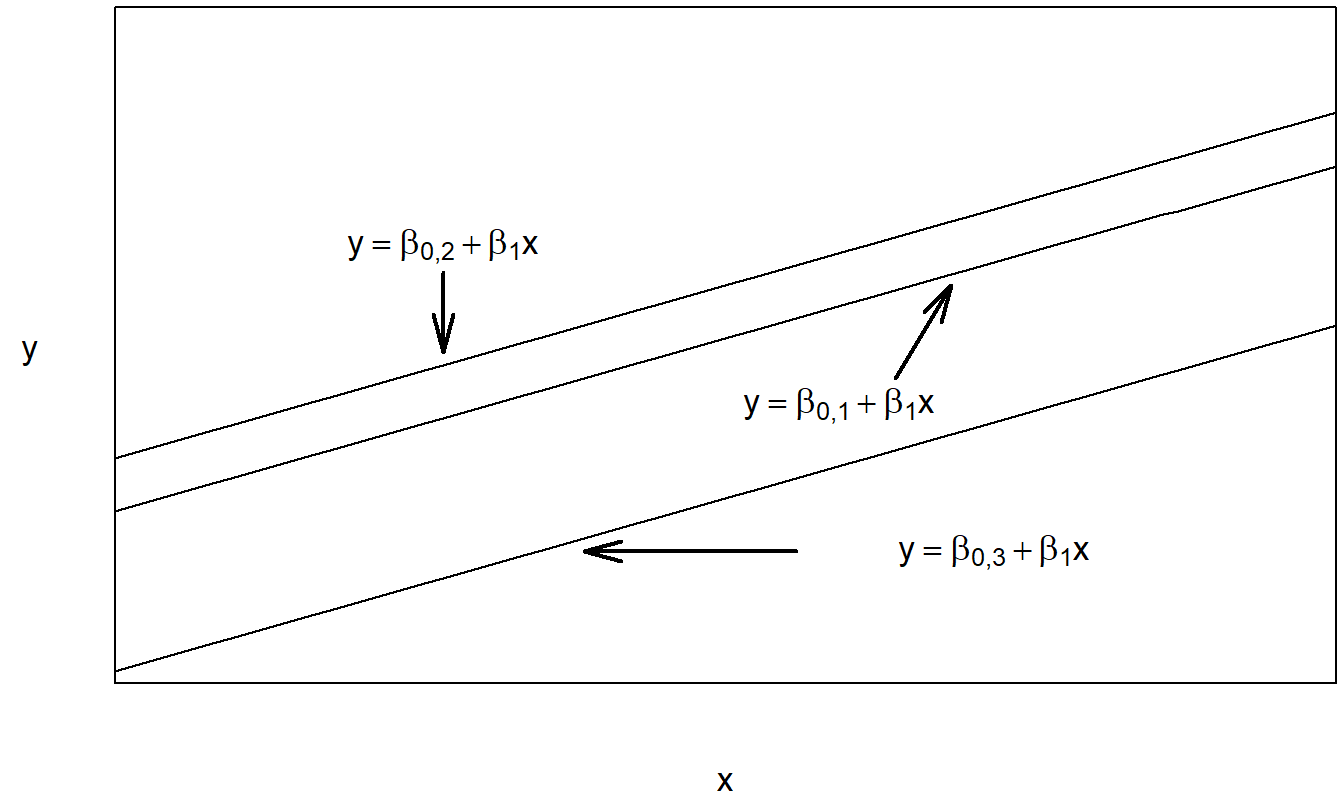
Figure 4.3: Plot of the expected response versus the covariate for the regression model with variable intercept and constant slope.

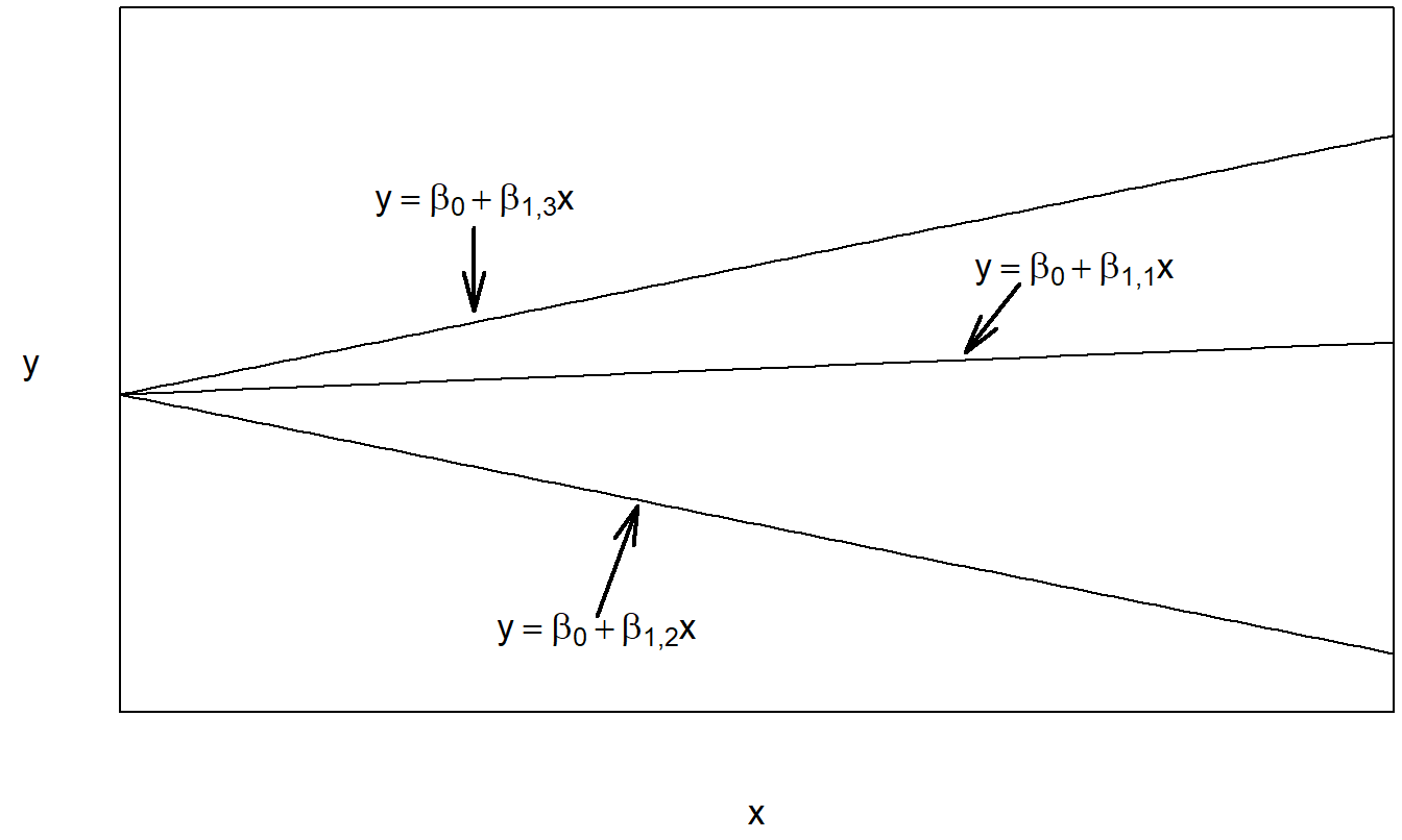
Figure 4.4: Plot of the expected response versus the covariate for the regression model with constant intercept and variable slope.

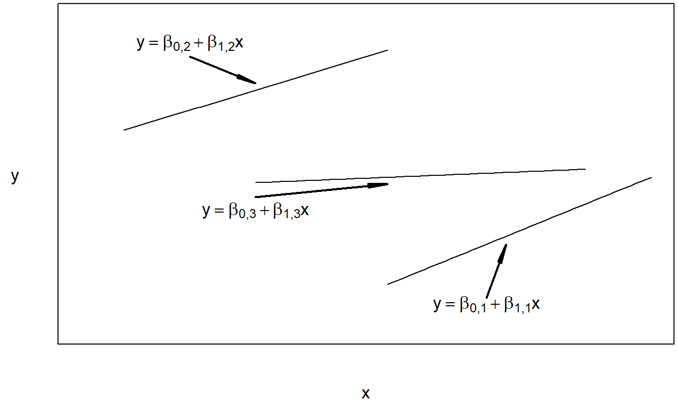
Figure 4.5: Plot of the expected response versus the covariate for the regression model with variable intercept and variable slope.

For each model presented in Table 4.8, parameter estimates can be calculated using the method of least squares. As usual, this means writing the expected response, \(E[y_{ij}]\), as a function of known variables and unknown parameters. For the regression model with variable intercept and constant slope, the least squares estimates can be expressed compactly as:

\[ b_1 = \frac{\sum_{j=1}^{c}\sum_{i=1}^{n_j} (x_{ij} - \bar{x}_j) (y_{ij} - \bar{y}_j)}{\sum_{j=1}^{c}\sum_{i=1}^{n_j} (x_{ij} - \bar{x}_j)^2} \]

and \(b_{0j} = \bar{y}_j - b_1 \bar{x}_j\). Similarly, the least squares estimates for the regression model with variable intercept and slope can be expressed as:

\[ b_{1j} = \frac{\sum_{i=1}^{n_j} (x_{ij} - \bar{x}_j) (y_{ij} - \bar{y}_j)}{\sum_{i=1}^{n_j} (x_{ij} - \bar{x}_j)^2} \]

and \(b_{0j} = \bar{y}_j - b_{1j} \bar{x}_j\). With these parameter estimates, fitted values may be calculated.

For each model, fitted values are defined to be the expected response with the unknown parameters replaced by their least squares estimates. For example, for the regression model with variable intercept and constant slope the fitted values are \(\hat{y}_{ij} = b_{0j} + b_1 x_{ij}.\)

---

Example: Wisconsin Hospital Costs. We now study the impact of various predictors on hospital charges in the state of Wisconsin. Identifying predictors of hospital charges can provide direction for hospitals, government, insurers, and consumers in controlling these variables, which in turn leads to better control of hospital costs. The data for the year 1989 were obtained from the Office of Health Care Information, Wisconsin’s Department of Health and Human Services. Cross-sectional data are used, which detail the 20 diagnosis-related group (DRG) discharge costs for hospitals in the state of Wisconsin, broken down into nine major health service areas and three types of payer (Fee for service, HMO, and other). Even though there are 540 potential DRG, area, and payer combinations (\(20 \times 9 \times 3 = 540\)), only 526 combinations were actually realized in the 1989 data set. Other predictor variables included the logarithm of the total number of discharges (NO DSCHG) and total number of hospital beds (NUM BEDS) for each combination. The response variable is the logarithm of total hospital charges per number of discharges (CHGNUM). To streamline the presentation, we now consider only costs associated with three diagnostic related groups (DRGs): DRG #209, DRG #391, and DRG #430.

The covariate, \(x\), is the natural logarithm of the number of discharges. In ideal settings, hospitals with more patients enjoy lower costs due to economies of scale. In non-ideal settings, hospitals may not have excess capacity and thus, hospitals with more patients have higher costs. One purpose of this analysis is to investigate the relationship between hospital costs and hospital utilization.

Recall that our measure of hospital charges is the logarithm of costs per discharge (\(y\)). The scatter plot in Figure 4.6 gives a preliminary idea of the relationship between \(y\) and \(x\). We note that there appears to be a negative relationship between \(y\) and \(x\).

The negative relationship between \(y\) and \(x\) suggested by Figure 4.6 is misleading and is induced by an omitted variable, the category of the cost (DRG). To see the joint effect of the categorical variable DRG and the continuous variable \(x\), in Figure 4.7 is a plot of \(y\) versus \(x\) where the plotting symbols are codes for the level of the categorical variable. From this plot, we see that the level of cost varies by level of the factor DRG. Moreover, for each level of DRG, the slope between \(y\) and \(x\) is either zero or positive. The slopes are not negative, as suggested by Figure 4.6.

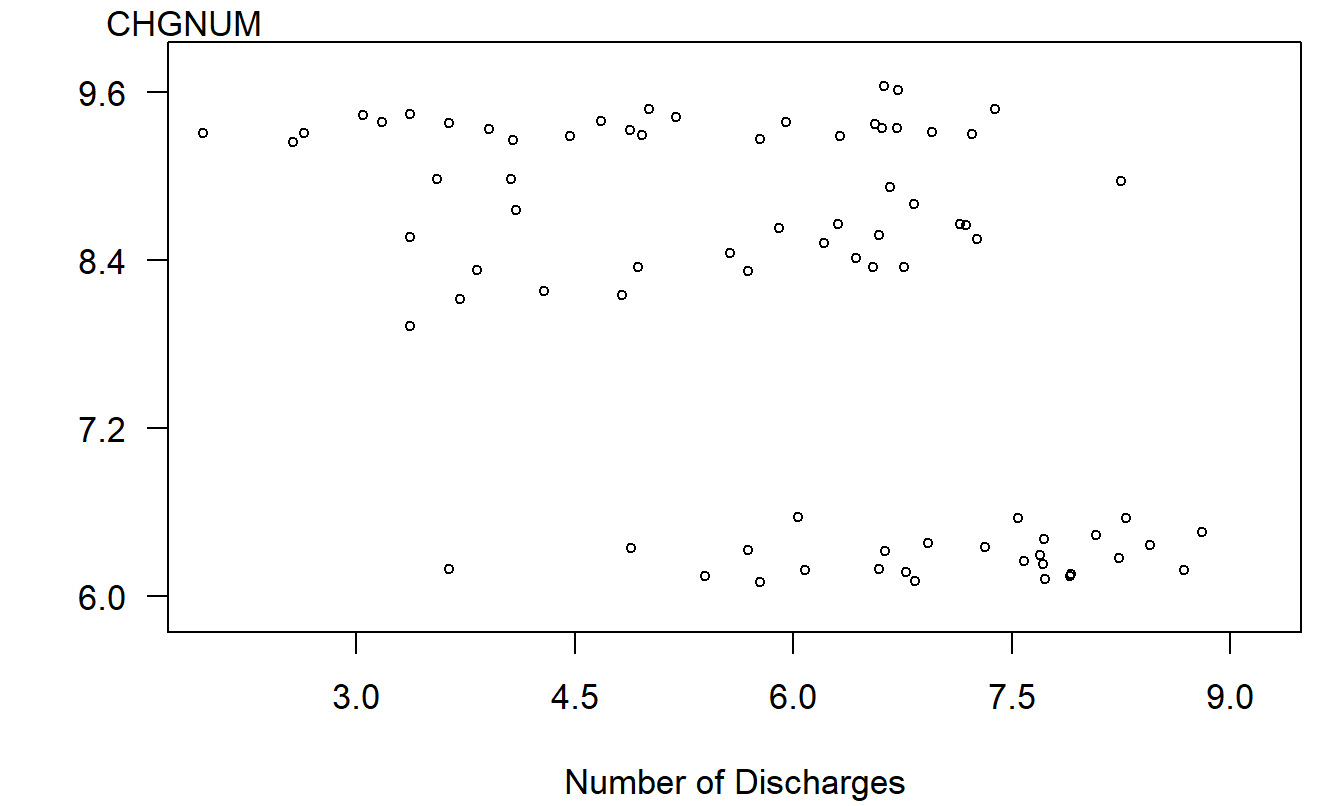
Figure 4.6: Plot of natural logarithm of cost per discharge versus natural logarithm of the number of discharges. This plot suggests a misleading negative relationship.

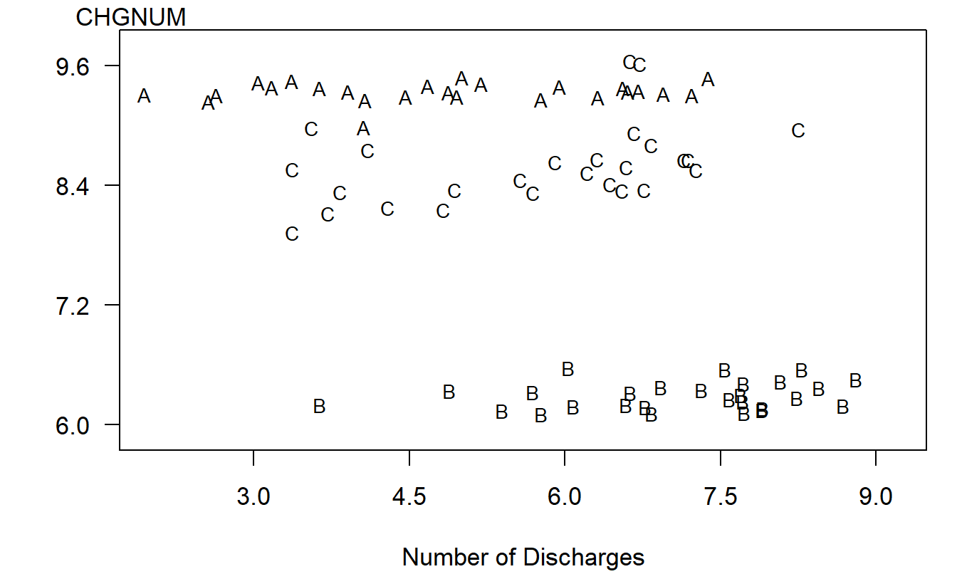
Figure 4.7: Letter plot of natural logarithm of cost per discharge versus natural logarithm of the number of discharges by DRG. Here, A is for DRG #209, B is for DRG #391, and C is for DRG #430.

Table 4.9: Wisconsin Hospital Cost Models Goodness of Fit

Model Description	Model degrees of freedom	Error degrees of freedom	Error Sum of Squares	R-squared (%)	Mean Square
One factor ANOVA	2	76	9.396	93.3	0.124
Regression with constant intercept and slope	1	77	115.059	18.2	1.222
Regression with variable intercept and constant slope	3	75	7.482	94.7	0.100
Regression with constant intercept and variable slope	3	75	14.048	90.0	0.187
Regression with variable intercept and slope	5	73	5.458	96.1	0.075

Each of the five models defined in Table 4.8 was fit to this subset of the Hospital case study. The summary statistics are in Table 4.9. For this data set, there are \(n = 79\) observations and \(c = 3\) levels of the DRG factor. For each model, the model degrees of freedom is the number of model parameters minus one. The error degrees of freedom is the number of observations minus the number of model parameters.

Using binary variables, each of the models in Table 4.8 can be written in a regression format. As we have seen in Section 4.2, when a model can be written as a subset of another, larger model, we have formal testing procedures available to decide which model is more appropriate. To illustrate this testing procedure with our DRG example, from Table 4.9 and the associated plots, it seems clear that the DRG factor is important. Further, a \(t\)-test, not presented here, shows that the covariate \(x\) is important. Thus, let’s compare the full model \(E[y_{ij}] = \beta_{0,j} + \beta_{1,j}x\) to the reduced model \(E[y_{ij}] = \beta_{0,j} + \beta_1x\). In other words, is there a different slope for each DRG?

Using the notation from Section 4.2, we call the variable intercept and slope the full model. Under the null hypothesis, \(H_0: \beta_{1,1} = \beta_{1,2} = \beta_{1,3}\), we get the variable intercept, constant slope model. Thus, using the \(F\)-ratio in equation (4.2), we have

\[ F\text{-ratio} = \frac{(Error~SS)_{reduced} - (Error~SS)_{full}}{ps_{full}^2} = \frac{7.482 - 5.458}{2 \times 0.075} = 13.535. \]

The 95th percentile from the \(F\)-distribution with \(df_1 = p = 2\) and \(df_2 = (df)_{full} = 73\) is approximately 3.13. Thus, this test leads us to reject the null hypothesis and declare the alternative, the regression model with variable intercept and variable slope, to be valid.

---

Combining Two Factors

We have seen how to combine covariates as well as a covariate and factor, both additively and with interactions. In the same fashion, suppose that we have two factors, say sex (two levels, male/female) and age (three levels, young/middle/old). Let the corresponding binary variables be \(x_1\) to indicate whether the observation represents a female, \(x_2\) to indicate whether the observation represents a young person, and \(x_3\) to indicate whether the observation represents a middle-aged person.

An additive model for these two factors may use the regression function

\[ \mathrm{E }~y = \beta_0 + \beta_1 x_1 + \beta_2 x_2 + \beta_3 x_3. \]

As we have seen, this model is simple to interpret. For example, we can interpret \(\beta_1\) to be the sex effect, holding age constant.

We can also incorporate two interaction terms, \(x_1 x_2\) and \(x_1 x_3\). Using all five explanatory variables yields the regression function

\[ \mathrm{E }~y = \beta_0 + \beta_1 x_1 + \beta_2 x_2 + \beta_3 x_3 + \beta_4 x_1 x_2 + \beta_5 x_1 x_3. \tag{4.12} \]

Here, the variables \(x_1\), \(x_2\), and \(x_3\) are known as the main effects. Table 4.10 helps interpret this equation. Specifically, there are six types of people that we could encounter: males and females who are young, middle-aged, or old. We have six parameters in equation (4.12). Table 4.10 provides the link between the parameters and the types of people. By using the interaction terms, we do not impose any prior specifications on the additive effects of each factor. From Table 4.10, we see that the interpretation of the regression coefficients in equation (4.12) is not straightforward. However, using the additive model with interaction terms is equivalent to creating a new categorical variable with six levels, one for each type of person. If the interaction terms are critical in your study, you may wish to create a new factor that incorporates the interaction terms simply for ease of interpretation.

Table 4.10: Regression Function for a Two Factor Model with Interactions

Sex	Age	\(x_1\)	\(x_2\)	\(x_3\)	\(x_4\)	\(x_5\)	Regression Function
Male	Young	0	1	0	0	0	\(\beta_0 + \beta_2\)
Male	Middle	0	0	1	0	0	\(\beta_0 + \beta_3\)
Male	Old	0	0	0	0	0	\(\beta_0\)
Female	Young	1	1	0	1	0	\(\beta_0 + \beta_1 + \beta_2 + \beta_4\)
Female	Middle	1	0	1	0	1	\(\beta_0 + \beta_1 + \beta_3 + \beta_5\)
Female	Old	1	0	0	0	0	\(\beta_0 + \beta_1\)

Extensions to more than two factors follow in a similar fashion. For example, suppose that you are examining the behavior of firms with headquarters in ten geographic regions, two organizational structures (profit versus non-profit) with four years of data. If you decide to treat each variable as a factor and want to model all interaction terms, then this is equivalent to a factor with \(10 \times 2 \times 4 = 80\) levels. Models with interaction terms can have a substantial number of parameters and the analyst must be prudent when specifying interactions to be considered.

General Linear Model

The general linear model extends the linear regression model in two ways. First, explanatory variables may be continuous, categorical, or a combination. The only restriction is that they enter linearly such that the resulting regression function

\[ \mathrm{E}~y = \beta_0 + \beta_1 x_1 + \ldots + \beta_k x_k \tag{4.13} \]

is a linear combination of coefficients. As we have seen, we can square continuous variables or take other nonlinear transforms (such as logarithms) as well as use binary variables to represent categorical variables, so this “restriction,” as the name suggests, allows for a broad class of general functions to represent data.

The second extension is that the explanatory variables may be linear combinations of one another in the general linear model. Because of this, in the general linear model case, the parameter estimates need not be unique. However, an important feature of the general linear model is that the resulting fitted values turn out to be unique, using the method of least squares.

For example, in Section 4.3 we saw that the one factor ANOVA model could be expressed as a regression model with \(c\) indicator variables. However, if we had attempted to estimate the model in equation (4.10), the method of least squares would not have arrived at a unique set of regression coefficient estimates. The reason is that, in equation (4.10), each explanatory variable can be expressed as a linear combination of the others. For example, observe that \(x_c = 1 - (x_1 + x_2 + \ldots + x_{c-1})\).

The fact that parameter estimates are not unique is a drawback, but not an overwhelming one. The assumption that the explanatory variables are not linear combinations of one another means that we can compute unique estimates of the regression coefficients using the method of least squares. In terms of matrices, because the explanatory variables are not linear combinations of one another, the matrix \(\mathbf{X}^{\prime}\mathbf{X}\) is not invertible.

Specifically, suppose that we are considering the regression function in equation (4.13) and, using the method of least squares, our regression coefficient estimates are \(b_0^{o}, b_1^{o}, \ldots, b_k^{o}\). This set of regression coefficient estimates minimizes our error sum of squares, but there may be other sets of coefficients that also minimize the error sum of squares. The fitted values are computed as \(\hat{y}_i = b_0^{o} + b_1^{o} x_{i1} + \ldots + b_k^{o} x_{ik}\). It can be shown that the resulting fitted values are unique, in the sense that any set of coefficients that minimize the error sum of squares produce the same fitted values (see Section 4.7.3).

Thus, for a set of data and a specified general linear model, fitted values are unique. Because residuals are computed as observed responses minus fitted values, we have that the residuals are unique. Because residuals are unique, we have the error sums of squares are unique. Thus, it seems reasonable, and is true, that we can use the general test of hypotheses described in Section 4.2 to decide whether collections of explanatory variables are important.

To summarize, for general linear models, parameter estimates may not be unique and thus not meaningful. An important part of regression models is the interpretation of regression coefficients. This interpretation is not necessarily available in the general linear model context. However, for general linear models, we may still discuss the importance of an individual variable or collection of variables through partial F-tests. Further, fitted values, and the corresponding exercise of prediction, works in the general linear model context. The advantage of the general linear model context is that we need not worry about the type of restrictions to impose on the parameters. Although not the subject of this text, this advantage is particularly important in complicated experimental designs used in the life sciences. The reader will find that general linear model estimation routines are widely available in statistical software packages available on the market today.

Video: Section Summary

4.5 Further Reading and References

There are several good linear model books that focus on categorical variables and analysis of variable techniques. Hocking (2003) and Searle (1987) are good examples.

Chapter References

• Hocking, Ronald R. (2003). Methods and Applications of Linear Models: Regression and the Analysis of Variance John Wiley and Sons, New York.
• Keeler, Emmett B., and John E. Rolph (1988). The demand for episodes of treatment in the Health Insurance Experiment. Journal of Health Economics 7: 337-367.
• Searle, Shayle R. (1987). Linear Models for Unbalanced Data. John Wiley & Sons, New York.

4.6 Exercises

4.1. In this exercise, we consider relating two statistics that summarize how well a regression model fits, the \(F\)-ratio and \(R^2\), the coefficient of determination. (Here, the \(F\)-ratio is the statistic used to test model adequacy, not a partial \(F\) statistic.)

1. Write down \(R^2\) in terms of \(Error ~SS\) and \(Regression ~SS\).
2. Write down \(F\)-ratio in terms of \(Error ~SS\), \(Regression ~SS\), \(k\), and \(n\).
3. Establish the algebraic relationship \[ F\text{-ratio} = \frac{R^2}{1-R^2} \frac{n-(k+1)}{k}. \]
4. Suppose that \(n = 40\), \(k = 5\), and \(R^2 = 0.20\). Calculate the \(F\)-ratio. Perform the usual test of model adequacy to determine whether or not the five explanatory variables jointly significantly affect the response variable.
5. Suppose that \(n = 400\) (not 40), \(k = 5\), and \(R^2 = 0.20\). Calculate the \(F\)-ratio. Perform the usual test of model adequacy to determine whether or not the five explanatory variables jointly significantly affect the response variable.

4.2. Hospital Costs. This exercise considers hospital expenditures data provided by the US Agency for Healthcare Research and Quality (AHRQ) and described in Exercise 1.4.

1. Produce a scatter plot, correlation, and a linear regression of \(LNTOTCHG\) on \(AGE\). Is \(AGE\) a significant predictor of \(LNTOTCHG\)?
2. You are concerned that newborns follow a different pattern than other ages. Create a binary variable that indicates whether or not \(AGE\) equals zero. Run a regression using this binary variable and \(AGE\) as explanatory variables. Is the binary variable statistically significant?
3. Now examine the gender effect, using the binary variable \(FEMALE\) that is one if the patient is female and zero otherwise. Run a regression using \(AGE\) and \(FEMALE\) as explanatory variables. Run a second regression including these two variables with an interaction term. Comment on whether the gender effect is important in either model.
4. Now consider the type of admission, \(APRDRG\), an acronym for “all patient refined diagnostic related group.” This is a categorical explanatory variable that provides information on the type of hospital admission. There are several hundred levels of this category. For example, level 640 represents admission for a normal newborn, with neonatal weight greater than or equal to 2.5 kilograms. As another example, level 225 represents admission resulting in an appendectomy.
   d(i). Run a one-factor ANOVA model, using \(APRDRG\) to predict \(LNTOTCHG\). Examine the \(R^2\) from this model and compare it to the coefficient of determination of the linear regression model of \(LNTOTCHG\) on \(AGE\). Based on this comparison, which model do you think is preferred?
   d(ii). For the one-factor model in part d(i), provide a 95% confidence interval for the mean of \(LNTOTCHG\) for level 225 corresponding to an appendectomy. Convert your final answer from logarithmic dollars to dollars via exponentiation.
   d(iii). Run a regression model of \(APRDRG\), \(FEMALE\), and \(AGE\) on \(LNTOTCHG\). State whether \(AGE\) is a statistically significant predictor of \(LNTOTCHG\). State whether \(FEMALE\) is a statistically significant predictor of \(LNTOTCHG\).

4.3. Nursing Home Utilization. This exercise considers nursing home data provided by the Wisconsin Department of Health and Family Services (DHFS) and described in Exercises 1.2, 2.10, and 2.20.

In addition to the size variables, we also have information on several binary variables. The variable \(URBAN\) is used to indicate the facility’s location. It is one if the facility is located in an urban environment and zero otherwise. The variable \(MCERT\) indicates whether the facility is Medicare-certified. Most, but not all, nursing homes are certified to provide Medicare-funded care. There are three organizational structures for nursing homes. They are government (state, counties, municipalities), for-profit businesses, and tax-exempt organizations. Periodically, facilities may change ownership and, less frequently, ownership type. We create two binary variables \(PRO\) and \(TAXEXEMPT\) to denote for-profit business and tax-exempt organizations, respectively. Some nursing homes opt not to purchase private insurance coverage for their employees. Instead, these facilities directly provide insurance and pension benefits to their employees; this is referred to as “self funding of insurance.” We use binary variable \(SELFFUNDINS\) to denote it.

You decide to examine the relationship between \(LOGTPY(y)\) and the explanatory variables. Use cost report year 2001 data, and do the following analysis.

1. There are three levels of organizational structures, but we only use two binary variables (\(PRO\) and \(TAXEXEMPT\)). Explain why.
2. Run a one-way analysis of variance using \(TAXEXEMPT\) as the factor. Decide whether or not tax-exempt is an important factor in determining \(LOGTPY\). State your null hypothesis, alternative hypothesis, and all components of the decision-making rule. Use a 5% level of significance.
3. Run a one-way analysis of variance using \(MCERT\) as the factor. Decide whether or not \(MCERT\) is an important factor in determining \(LOGTPY\).
   c(i). Provide a point estimate of \(LOGTPY\) for a nursing facility that is not Medicare-Certified.
   c(ii). Provide a 95% confidence interval for your point estimate in part (i).
   
4. Run a regression model using the binary variables, \(URBAN\), \(PRO\), \(TAXEXEMPT\), \(SELFFUNDINS\), and \(MCERT\). Find \(R^2\). Which variables are statistically significant?
5. Run a regression model using all explanatory variables, \(LOGNUMBED\), \(LOGSQRFOOT\), \(URBAN\), \(PRO\), \(TAXEXEMPT\), \(SELFFUNDINS\), and \(MCERT\). Find \(R^2\). Which variables are statistically significant?
   e(i). Calculate the partial correlation between \(LOGTPY\) and \(LOGSQRFOOT\). Compare this to the correlation between \(LOGTPY\) and \(LOGSQRFOOT\). Explain why the partial correlation is small.
   e(ii). Compare the low level of the \(t\)-ratios (for testing the importance of individual regression coefficients) and the high level of the \(F\)-ratio (for testing model adequacy). Describe the seeming inconsistency and provide an explanation for this inconsistency.

4.4. Automobile Insurance Claims. Refer to Exercise 1.3.

1. Run a regression of \(LNPAID\) on \(AGE\). Is \(AGE\) a statistically significant variable? To respond to this question, use a formal test of hypothesis. State your null and alternative hypotheses, decision-making criterion, and your decision-making rule. Also comment on the goodness of fit of this variable.
2. Consider using class as a single explanatory variable. Use the one factor to estimate the model and respond to the following questions.
   b(i). What is the point estimate of claims in class C7, drivers 50-69, driving to work or school, less than 30 miles per week with annual mileage under 7500, in natural logarithmic units?
   b(ii). Determine the corresponding 95% confidence interval of expected claims, in natural logarithmic units.
   b(iii). Convert the 95% confidence interval of expected claims that you determined in part b(ii) to dollars.
   
3. Run a regression of \(LNPAID\) on \(AGE\), \(GENDER\), and the categorical variables \(STATE\ CODE\) and \(CLASS\).
   c(i). Is \(GENDER\) a statistically significant variable? To respond to this question, use a formal test of hypothesis. State your null and alternative hypotheses, decision-making criterion, and your decision-making rule.
   c(ii). Is \(CLASS\) a statistically significant variable? To respond to this question, use a formal test of hypothesis. State your null and alternative hypotheses, decision-making criterion, and your decision-making rule.
   c(iii). Use the model to provide a point estimate of claims in dollars (not log dollars) for a male age 60 in STATE 2 in CLASS C7.
   c(iv). Write down the coefficient associated with CLASS C7 and interpret this coefficient.

4.5. Wisconsin Lottery Sales. This exercise considers State of Wisconsin lottery sales data that were described in Section 2.1 and examined in Exercise 3.4.

Part 1: You decide to examine the relationship between SALES (\(y\)) and all eight explanatory variables (\(PERPERHH\), \(MEDSCHYR\), \(MEDHVL\), \(PRCRENT\), \(PRC55P\), \(HHMEDAGE\), \(MEDINC\), and \(POP\)).

1. Fit a regression model of SALES on all eight explanatory variables.

2. Find \(R^2\).
   b(i). Use it to calculate the correlation coefficient between the observed and fitted values.
   b(ii). You want to use \(R^2\) to test the adequacy of the model in part (a). Use a formal test of hypothesis. State your null and alternative hypothesis, decision-making criterion, and your decision-making rules.
   

3. Test whether \(POP\), \(MEDSCHYR\), and \(MEDHVL\) are jointly important explanatory variables for understanding SALES.

   Part 2: After the preliminary analysis in Part 1, you decide to examine the relationship between SALES (\(y\)) and \(POP\), \(MEDSCHYR\), and \(MEDHVL\).

   1. Fit a regression model of SALES on these three explanatory variables.

   2. Has the coefficient of determination decreased from the eight-variable regression model to the three-variable model? Does this mean that the model is not improved or does it provide little information? Explain your response.

   3. To state formally whether one should use the three or eight variable model, use a partial \(F\)-test. State your null and alternative hypotheses, decision-making criterion, and your decision-making rules.

4.6. Insurance Company Expenses. This exercise considers insurance company data from the NAIC and described in Exercises 1.6 and 3.5.

1. Are the quadratic terms important?

Consider a linear model of \(LNEXPENSES\) on twelve explanatory variables. For the explanatory variables, include \(ASSETS\), \(GROUP\), both versions of losses and gross premiums, as well as the two BLS variables. Also include the square of each of the two loss and the two gross premium variables.

Test whether the four squared terms are jointly statistically significant, using a partial \(F\)-test. State your null and alternative hypotheses, decision-making criterion, and your decision-making rules.

2. Are the interaction terms with \(GROUP\) important?

Omit the two BLS variables, so that now there are eleven variables: \(ASSETS\), \(GROUP\), both versions of losses and gross premiums, as well as interactions of \(GROUP\) with \(ASSETS\) and both versions of losses and gross premiums.

Test whether the five interaction terms are jointly statistically significant, using a partial \(F\)-test. State your null and alternative hypotheses, decision-making criterion, and your decision-making rules.

3. You are examining a company that is not in the sample with values \(LONGLOSS = 0.025\), \(SHORTLOSS = 0.040\), \(GPWPERSONAL = 0.050\), \(GPWCOMM = 0.120\), \(ASSETS = 0.400\), \(CASH = 0.350\), and \(GROUP = 1\).

Use the eleven variable interaction model in part (b) to produce a 95% prediction interval for this company.

4.7. National Life Expectancies. We continue the analysis begun in Exercises 1.7, 2.22, and 3.6.

1. Consider the regression using three explanatory variables, \(FERTILITY\), \(PUBLICEDUCATION\), and \(\ln{HEALTH}\) that you did in Exercise 3.6. Test whether \(PUBLICEDUCATION\) and \(\ln{HEALTH}\) are jointly statistically significant, using a partial \(F\)-test. State your null and alternative hypotheses, decision-making criterion, and your decision-making rules. (Hint: Use the coefficient of determination form for calculating the test statistic.) Provide an approximate \(p\)-value for the test.
2. We now introduce the \(REGION\) variable, summarized in Table 4.11. A boxplot of life expectancies versus \(REGION\) is given in Figure 4.8. Describe what we learn from the Table and boxplot about the effect of \(REGION\) on \(LIFEEXP\).

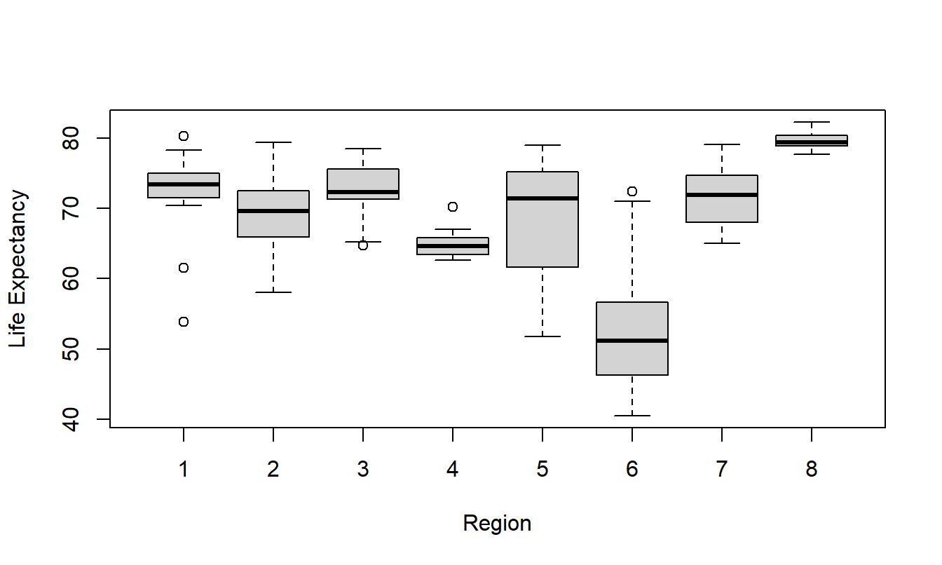
Figure 4.8: Boxplots of LIFEEXP by REGION

Table 4.11: Average Life Expectancy by Region

Region	Description of the Region	Number	Mean
1	Arab States	13	71.9
2	East Asia and the Pacific	17	69.1
3	Latin American and the Carribean	25	72.8
4	South Asia	7	65.1
5	Southern Europe	3	67.4
6	Sub-Saharan Africa	38	52.2
7	Central and Eastern Europe	24	71.6
8	High Income OECD	23	79.6
	All	150	67.4

Table 4.11 summarizes average life expectancy by region.

REGION	Region Description	Number	Mean
1	Arab States	13	71.9
2	East Asia and the Pacific	17	69.1
3	Latin American and the Carribean	25	72.8
4	South Asia	7	65.1
5	Southern Europe	3	67.4
6	Sub-Saharan Africa	38	52.2
7	Central and Eastern Europe	24	71.6
8	High Income OECD	23	79.6
	All	150	67.4

3. Fit a regression model using only the factor, \(REGION\). Is \(REGION\) a statistically significant determinant of \(LIFEEXP\)? State your null and alternative hypotheses, decision-making criterion, and your decision-making rules.
4. Fit a regression model using three explanatory variables, \(FERTILITY\), \(PUBLICEDUCATION\), and \(\ln{HEALTH}\), as well as the categorical variable \(REGION\).
   d(i). You are examining a country not in the sample with values \(FERTILITY = 2.0\), \(PUBLICEDUCATION = 5.0\), and \(\ln{HEALTH} = 1.0\). Produce two predicted life expectancy values by assuming that the country is from (1) an Arab state and (2) Sub-Saharan Africa.
   d(ii). Provide a 95% confidence interval for the difference in life expectancies between an Arab state and a country from Sub-Saharan Africa.
   d(iii). Provide the (usual ordinary least squares) point estimate for the difference in life expectancies between a country from Sub-Saharan Africa and a high-income OECD (Organization for Economic Co-operation and Development) country.

4.7 Technical Supplement - Matrix Expressions

4.7.1 Expressing Models with Categorical Variables in Matrix Form

Chapter 3 showed how to write the regression model equation in the form \(\mathbf{y = X} \boldsymbol{\beta} + \boldsymbol{\varepsilon}\) where \(\mathbf{X}\) is a matrix of explanatory variables. This form permits straightforward calculation of regression coefficients, \(\mathbf{b} = \left(\mathbf{X}^{\prime} \mathbf{X}\right)^{-1} \mathbf{X}^{\prime} \mathbf{y}\). This section shows how the model and calculations reduce to simpler expressions when the explanatory variables are categorical.

One Categorical Variable Model. Consider the model with one categorical variable introduced in Section 4.3 with \(c\) levels of the categorical variable. From equation (4.9), this model can be written as

\[ \mathbf{y} = \begin{bmatrix} y_{1,1} \\ \cdot \\ \cdot \\ \cdot \\ y_{n_1,1} \\ \cdot \\ \cdot \\ \cdot \\ y_{1,c} \\ \cdot \\ \cdot \\ \cdot \\ y_{n_{c},c} \end{bmatrix} = \begin{bmatrix} 1 & 0 & \cdots & 0 \\ \cdot & \cdot & \cdots & \cdot \\ \cdot & \cdot & \cdots & \cdot \\ \cdot & \cdot & \cdots & \cdot \\ 1 & 0 & \cdots & \cdots \\ \cdot & \cdot & \cdots & \cdot \\ \cdot & \cdot & \cdots & \cdot \\ \cdot & \cdot & \cdots & \cdot \\ 0 & 0 & \cdots & 1 \\ \cdot & \cdot & \cdots & \cdot \\ \cdot & \cdot & \cdots & \cdot \\ \cdot & \cdot & \cdots & \cdot \\ 0 & 0 & \cdots & 1 \\ \end{bmatrix} \begin{bmatrix} \mu_1 \\ \cdot \\ \cdot \\ \cdot \\ \mu_c \end{bmatrix} + \begin{bmatrix} \varepsilon_{1,1} \\ \cdot \\ \cdot \\ \cdot \\ \varepsilon_{n_1,1} \\ \cdot \\ \cdot \\ \cdot \\ \varepsilon_{1,c} \\ \cdot \\ \cdot \\ \cdot \\ \varepsilon_{n_{c},c} \end{bmatrix} = \mathbf{X} \boldsymbol{\beta} + \boldsymbol{\varepsilon} \]

To make the notation more compact, we write \(\mathbf{0}\) and \(\mathbf{1}\) for a column of zeros and ones, respectively. With this convention, another way to express this as

\[ \mathbf{y} = \begin{bmatrix} \mathbf{1}_1 & \mathbf{0}_1 & \cdots & \mathbf{0}_1 \\ \mathbf{0}_2 & \mathbf{1}_2 & \cdots & \mathbf{0}_2 \\ \vdots & \vdots & \ddots & \vdots \\ \mathbf{0}_c & \mathbf{0}_c & \cdots & \mathbf{1}_c \end{bmatrix} \begin{bmatrix} \mu_1 \\ \mu_2 \\ \vdots \\ \mu_c \end{bmatrix} + \boldsymbol{\varepsilon} = \mathbf{X} \boldsymbol{\beta} + \boldsymbol{\varepsilon} \tag{4.14} \]

Here, \(\mathbf{0}_1\) and \(\mathbf{1}_1\) stand for vector columns of length \(n_1\) of zeros and ones, respectively, and similarly for \(\mathbf{0}_2, \mathbf{1}_2, \ldots, \mathbf{0}_c, \mathbf{1}_c\).

Equation (4.14) allows us to apply the machinery developed for the regression model to the model with one categorical variable. As an intermediate calculation, we have

\[ \begin{array}{ll} (\mathbf{X}^{\prime} \mathbf{X})^{-1} &= \left( \begin{bmatrix} \mathbf{1}_1 & \mathbf{0}_2 & \cdots & \mathbf{0}_c \\ \mathbf{0}_1 & \mathbf{1}_2 & \cdots & \mathbf{0}_c \\ \vdots & \vdots & \ddots & \vdots \\ \mathbf{0}_1 & \mathbf{0}_2 & \cdots & \mathbf{1}_c \end{bmatrix}^{\prime} \begin{bmatrix} \mathbf{1}_1 & \mathbf{0}_1 & \cdots & \mathbf{0}_1 \\ \mathbf{0}_2 & \mathbf{1}_2 & \cdots & \mathbf{0}_2 \\ \vdots & \vdots & \ddots & \vdots \\ \mathbf{0}_c & \mathbf{0}_c & \cdots & \mathbf{1}_c \end{bmatrix} \right)^{-1}\\ &= \begin{bmatrix} n_1 & 0 & \cdots & 0 \\ 0 & n_2 & \cdots & 0 \\ \vdots & \vdots & \ddots & \vdots \\ 0 & 0 & \cdots & n_c \end{bmatrix}^{-1} = \begin{bmatrix} \frac{1}{n_1} & 0 & \cdots & 0 \\ 0 & \frac{1}{n_2} & \cdots & 0 \\ \vdots & \vdots & \ddots & \vdots \\ 0 & 0 & \cdots & \frac{1}{n_c} \end{bmatrix} . \tag{4.15} \end{array} \]

Thus, the parameter estimates are

\[ \mathbf{b} = \begin{bmatrix} \hat{\mu}_1 \\ \vdots \\ \hat{\mu}_c \end{bmatrix} = (\mathbf{X}^{\prime} \mathbf{X})^{-1} \mathbf{X}^{\prime} \mathbf{y} = \begin{bmatrix} \frac{1}{n_1} & 0 & \cdots & 0 \\ 0 & \frac{1}{n_2} & \cdots & 0 \\ \vdots & \vdots & \ddots & \vdots \\ 0 & 0 & \cdots & \frac{1}{n_c} \end{bmatrix} \begin{bmatrix} \mathbf{1}_1 & \mathbf{0}_2 & \cdots & \mathbf{0}_c \\ \mathbf{0}_1 & \mathbf{1}_2 & \cdots & \mathbf{0}_c \\ \vdots & \vdots & \ddots & \vdots \\ \mathbf{0}_1 & \mathbf{0}_2 & \cdots & \mathbf{1}_c \end{bmatrix}^{\prime} \begin{bmatrix} y_{1,1} \\ \vdots \\ y_{n_1,1} \\ \vdots \\ y_{1,c} \\ \vdots \\ y_{n_{c},c} \end{bmatrix} \]

\[ = \begin{bmatrix} \frac{1}{n_1} & 0 & \cdots & 0 \\ 0 & \frac{1}{n_2} & \cdots & 0 \\ \vdots & \vdots & \ddots & \vdots \\ 0 & 0 & \cdots & \frac{1}{n_c} \end{bmatrix} \begin{bmatrix} \sum_{i=1}^{n_1} y_{i1} \\ \vdots \\ \sum_{i=1}^{n_c} y_{ic} \end{bmatrix} = \begin{bmatrix} \bar{y}_1 \\ \vdots \\ \bar{y}_c \end{bmatrix} \tag{4.16} \]

We have seen that the least squares estimate of \(\mu_j\), \(\bar{y}_j\), can been obtained directly from equation (4.9). By rewriting the model in matrix regression notation, we can appeal to linear regression model results and need not prove properties of models with categorical variables from first principles. That is, because this model is in regression format, we immediately have all the properties of the regression model.

Telling your software package that a variable is categorical can mean more efficient calculations, as in the calculations of the least squares regression estimates in equation (4.16). Further, calculation of other quantities can also be done more directly. As another example, we have that the standard error of \(\hat{\mu}_j\) is

\[ se(\hat{\mu}_j) = s ~ \sqrt{j \text{th} \textit{ diagonal element of } \mathbf{(X}^{\prime}\mathbf{X)}^{-1}} = s/\sqrt{n_j}. \]

One Categorical and One Continuous Variable Model

As another illustration, we consider the variable intercept and constant slope model. This model is summarized as \(\mathbf{y} = \mathbf{X} \boldsymbol \beta + \boldsymbol \varepsilon\) where

\[ \mathbf{X} = \begin{bmatrix} \mathbf{1}_1 & \mathbf{0}_1 & \cdot \cdot \cdot & \mathbf{0}_1 & \mathbf{x}_1 \\ \mathbf{0}_2 & \mathbf{1}_2 & \cdot \cdot \cdot & \mathbf{0}_2 & \mathbf{x}_2 \\ \cdot & \cdot & \cdot \cdot \cdot & \cdot & \cdot \\ \cdot & \cdot & \cdot \cdot \cdot & \cdot & \cdot \\ \cdot & \cdot & \cdot \cdot \cdot & \cdot & \cdot \\ \mathbf{0}_{c} & \mathbf{0}_{c} & \cdot \cdot \cdot & \mathbf{1}_c & \mathbf{x}_{c} \end{bmatrix} \text{ and } \boldsymbol \beta = \begin{bmatrix} \beta_{01} \\ \beta_{02} \\ \cdot \\ \cdot \\ \cdot \\ \beta_{0c} \\ \beta_1 \end{bmatrix}. \tag{4.17} \]

Here, \(\mathbf{0}_j\) and \(\mathbf{1}_j\) stand for vector columns of length \(n_j\) of zeros and ones, respectively, and \(\mathbf{x}_j = (x_{1j}, x_{2j}, \ldots, x_{n_j, j})^{\prime}\) is the column of the continuous variable at the \(j\)th level. Straightforward matrix algebra techniques provide the least squares estimates.

4.7.2 Calculating Least Squares Recursively

When computing regression coefficients using least squares, \(\mathbf{b} = \left(\mathbf{X}^{\prime} \mathbf{X}\right)^{-1} \mathbf{X}^{\prime} \mathbf{y}\), for some applications, the dimension of \(\mathbf{X}^{\prime} \mathbf{X}\) can be large, causing computational difficulties. Fortunately, for some problems, the computations can be partitioned into smaller problems that can be solved recursively.

Recursive Least Squares Calculation. Suppose that the regression function can be written as

\[ \mathrm{E}~\mathbf{y} = \mathbf{X} \boldsymbol \beta = \left( \mathbf{X}_1 : \mathbf{X}_2 \right) \left( \begin{array}{c} \boldsymbol \beta_1 \\ \boldsymbol \beta_2 \\ \end{array} \right), \tag{4.18} \]

where \(\mathbf{X}_1\) has dimensions \(n \times k_1\), \(\mathbf{X}_2\) has dimensions \(n \times k_2\), \(k_1 + k_2 = k\), \(\boldsymbol \beta_1\) has dimensions \(k_1 \times 1\), and \(\boldsymbol \beta_2\) has dimensions \(k_2 \times 1\). Define \(\mathbf{Q}_1 = \mathbf{I} - \mathbf{X}_1 \left(\mathbf{X}_1^{\prime} \mathbf{X}_1\right)^{-1} \mathbf{X}_1^{\prime}\). Then, the least squares estimator can be computed as:

\[ \mathbf{b} = \left( \begin{array}{c} \mathbf{b}_1 \\ \mathbf{b}_2 \\ \end{array} \right) = \left( \begin{array}{c} (\mathbf{X}_1^{\prime} \mathbf{X}_1)^{-1} \mathbf{X}_1^{\prime} \left( \mathbf{y} - \mathbf{X}_2 \mathbf{b}_2 \right) \\ \left(\mathbf{X}_2^{\prime} \mathbf{Q}_1 \mathbf{X}_2\right)^{-1} \mathbf{X}_2^{\prime} \mathbf{Q}_1 \mathbf{y} \\ \end{array} \right). \tag{4.19} \]

Equation (4.19) provides the first step in the recursion. It can easily be iterated to allow for a more detailed decomposition of \(\mathbf{X}\).

Special Case: One Categorical and One Continuous Variable Model. To illustrate the relevance of equation (4.19), consider the model summarized in equation (4.17). Here, the dimension of \(\mathbf{X}\) is \(n \times (c+1)\) and so the dimension of \(\mathbf{X}^{\prime} \mathbf{X}\) is \((c+1) \times (c+1)\). Taking the inverse of this matrix could be difficult if \(c\) is large. To apply equation (4.19), we define

\[ \mathbf{X}_1 = \begin{bmatrix} \mathbf{1}_1 & \mathbf{0}_1 & \cdot \cdot \cdot & \mathbf{0}_1 \\ \mathbf{0}_2 & \mathbf{1}_2 & \cdot \cdot \cdot & \mathbf{0}_2 \\ \cdot & \cdot & \cdot \cdot \cdot & \cdot \\ \cdot & \cdot & \cdot \cdot \cdot & \cdot \\ \cdot & \cdot & \cdot \cdot \cdot & \cdot \\ \mathbf{0}_c & \mathbf{0}_c & \cdot \cdot \cdot & \mathbf{1}_c \end{bmatrix} \text{ and } \mathbf{X}_2 = \begin{bmatrix} \mathbf{x}_1 \\ \mathbf{x}_2 \\ \cdot \\ \cdot \\ \cdot \\ \mathbf{x}_c \end{bmatrix}. \]

In this case, we have seen in equation (4.15) how it is straightforward to compute \(\left(\mathbf{X}_1^{\prime} \mathbf{X}_1\right)^{-1}\) without requiring matrix inversion. This makes calculating \(\mathbf{Q}_1\) straightforward. With this, we can compute \(\mathbf{X}_2^{\prime} \mathbf{Q}_1 \mathbf{X}_2\) and, because it is a scalar, immediately get its inverse. This provides \(\mathbf{b}_2\) which is then used to calculate \(\mathbf{b}_1\). Although this procedure is not as direct as \(\mathbf{b} = \left(\mathbf{X}^{\prime} \mathbf{X}\right)^{-1} \mathbf{X}^{\prime} \mathbf{y}\), it can be computationally efficient.

Partitioned Matrix Results

To establish equation (4.19), we use results standard in matrix algebra regarding the inverses of partitioned matrices.

Partitioned Matrix Results. Suppose that we can partition the \((p+q) \times (p+q)\) matrix \(\mathbf{B}\) as

\[ \mathbf{B} = \begin{bmatrix} \mathbf{B}_{11} & \mathbf{B}_{12} \\ \mathbf{B}_{12}^{\prime} & \mathbf{B}_{22} \end{bmatrix}, \]

where \(\mathbf{B}_{11}\) is a \(p \times p\) invertible matrix, \(\mathbf{B}_{22}\) is a \(q \times q\) invertible matrix, and \(\mathbf{B}_{12}\) is a \(p \times q\) matrix. Then

\[ \mathbf{B}^{-1} = \begin{bmatrix} \mathbf{C}_{11}^{-1} & - \mathbf{B}_{11}^{-1} \mathbf{B}_{12} \mathbf{C}_{22}^{-1} \\ - \mathbf{C}_{22}^{-1} \mathbf{B}_{12}^{\prime} \mathbf{B}_{11}^{-1} & \mathbf{C}_{22}^{-1} \end{bmatrix}, \tag{4.20} \]

where \(\mathbf{C}_{11} = \mathbf{B}_{11} - \mathbf{B}_{12} \mathbf{B}_{22}^{-1} \mathbf{B}_{12}^{\prime}\) and \(\mathbf{C}_{22} = \mathbf{B}_{22} - \mathbf{B}_{12}^{\prime} \mathbf{B}_{11}^{-1} \mathbf{B}_{12}.\)

To verify equation (4.20), multiply \(\mathbf{B}^{-1}\) by \(\mathbf{B}\) to obtain the identity matrix \(\mathbf{I}\). Further,

\[ \mathbf{C}_{11}^{-1} = \mathbf{B}_{11}^{-1} + \mathbf{B}_{11}^{-1} \mathbf{B}_{12} \mathbf{C}_{22}^{-1} \mathbf{B}_{12}^{\prime} \mathbf{B}_{11}^{-1}. \tag{4.21} \]

Now, we first write the least squares estimator as \[ \begin{array}{ll} \mathbf{b} &= \left( \mathbf{X}^{\prime}\mathbf{X}\right)^{-1} \mathbf{X}^{\prime} \mathbf{y} = \left( \left( \begin{array}{c} \mathbf{X}_1^{\prime} \\ \mathbf{X}_2^{\prime} \\ \end{array} \right) \left( \mathbf{X}_1 : \mathbf{X}_2 \right)\right)^{-1} \left( \begin{array}{c} \mathbf{X}_1^{\prime} \\ \mathbf{X}_2^{\prime} \\ \end{array} \right) \mathbf{y} \\ & = \left( \begin{array}{cc} \mathbf{X}_1^{\prime} \mathbf{X}_1 & \mathbf{X}_1^{\prime} \mathbf{X}_2 \\ \mathbf{X}_2^{\prime} \mathbf{X}_1 & \mathbf{X}_2^{\prime} \mathbf{X}_2 \\ \end{array} \right)^{-1} \left( \begin{array}{c} \mathbf{X}_1^{\prime} \mathbf{y} \\ \mathbf{X}_2^{\prime} \mathbf{y} \\ \end{array} \right) = \left( \begin{array}{c} \mathbf{b}_1 \\ \mathbf{b}_2 \\ \end{array} \right). \end{array} \] To apply the partitioned matrix results, we define \[ \mathbf{Q}_j = \mathbf{I} - \mathbf{X}_j \left(\mathbf{X}_j^{\prime}\mathbf{X}_j \right)^{-1} \mathbf{X}_j^{\prime}, \] \(j=1,2,\) and \(\mathbf{B}_{j,k} = \mathbf{X}_j^{\prime}\mathbf{X}_k\) for \(j,k=1,2.\) This means that \(\mathbf{C}_{11}=\mathbf{X}_1^{\prime}\mathbf{X}_1 - \mathbf{X}_1^{\prime}\mathbf{X}_2 (\mathbf{X}_2^{\prime}\mathbf{X}_2)^{-1} \mathbf{X}_2^{\prime}\mathbf{X}_1^{\prime }\) \(= \mathbf{X}_1^{\prime} \mathbf{Q}_2 \mathbf{X}_1\) and similarly \(\mathbf{C}_{22} = \mathbf{X}_2^{\prime} \mathbf{Q}_1 \mathbf{X}_2\). From the second row, we have \[ \begin{array}{ll} \mathbf{b}_2 &= \mathbf{C}_{22}^{-1} \left( -\mathbf{B}_{12}^{\prime} \mathbf{B}_{11}^{-1}\mathbf{X}_1^{\prime} \mathbf{y} + \mathbf{X}_2^{\prime} \mathbf{y} \right) \\ &= \left(\mathbf{X}_2^{\prime} \mathbf{Q}_1 \mathbf{X}_2 \right)^{-1} \left( - \mathbf{X}_2^{\prime} \mathbf{X}_1 (\mathbf{X}_1^{\prime}\mathbf{X}_1)^{-1} \mathbf{X}_1^{\prime} \mathbf{y} + \mathbf{X}_2^{\prime}\mathbf{y} \right) \\ &= \left(\mathbf{X}_2^{\prime} \mathbf{Q}_1 \mathbf{X}_2 \right)^{-1} \mathbf{X}_2^{\prime} \mathbf{Q}_1\mathbf{y}. \end{array} \]

From the first row,

\[ \begin{array}{ll} \mathbf{b}_1 &= \mathbf{C}_{11}^{-1} \mathbf{X}_1^{\prime}\mathbf{y} - \mathbf{B}_{11}^{-1}\mathbf{B}_{12}\mathbf{C}_{22}^{-1} \mathbf{X}_2^{\prime}\mathbf{y} \\ &= \left( \mathbf{B}_{11}^{-1} + \mathbf{B}_{11}^{-1} \mathbf{B}_{12} \mathbf{C}_{22}^{-1} \mathbf{B}_{21} \mathbf{B}_{11}^{-1} \right) \mathbf{X}_1^{\prime}\mathbf{y} - \mathbf{B}_{11}^{-1}\mathbf{B}_{12}\mathbf{C}_{22}^{-1} \mathbf{X}_2^{\prime}\mathbf{y} \\ &= \mathbf{B}_{11}^{-1}\mathbf{X}_1^{\prime}\mathbf{y} - \mathbf{B}_{11}^{-1} \mathbf{B}_{12} \mathbf{C}_{22}^{-1} \left( -\mathbf{B}_{21} \mathbf{B}_{11}^{-1} \mathbf{X}_1^{\prime}\mathbf{y} + \mathbf{X}_2^{\prime}\mathbf{y} \right)\\ &= \mathbf{B}_{11}^{-1}\mathbf{X}_1^{\prime}\mathbf{y} - \mathbf{B}_{11}^{-1} \mathbf{B}_{12} \mathbf{b}_2 \\ &= (\mathbf{X}_1^{\prime}\mathbf{X}_1)^{-1}\mathbf{X}_1^{\prime}\mathbf{y} - (\mathbf{X}_1^{\prime}\mathbf{X}_1)^{-1} \mathbf{X}_1^{\prime}\mathbf{X}_2 \mathbf{b}_2 \\ &= (\mathbf{X}_1^{\prime}\mathbf{X}_1)^{-1}\mathbf{X}_1^{\prime} \left( \mathbf{y} - \mathbf{X}_2 \mathbf{b}_2 \right). \end{array} \]

This establishes equation (4.19).

Reparameterized Model. For the partitioned regression function in equation (4.18), define \(\mathbf{A}= \left( \mathbf{X}_1^{\prime} \mathbf{X}_1 \right)^{-1} \mathbf{X}_1^{\prime} \mathbf{X}_2\) and \(\mathbf{E}_2 = \mathbf{X}_2 - \mathbf{X}_1 \mathbf{A}\). If one were to run a “multivariate” regression using \(\mathbf{X}_2\) as the response and \(\mathbf{X}_1\) as explanatory variables, then the parameter estimates would be \(\mathbf{A}\) and the residuals \(\mathbf{E}_2\).

With these definitions, use equation (4.18) to define the reparameterized regression model \[ \begin{array}{ll} \mathbf{y} & = \mathbf{X}_1 \boldsymbol \beta_1 + \mathbf{X}_2 \boldsymbol \beta_2 + \boldsymbol \varepsilon = \mathbf{X}_1 \boldsymbol \beta_1 + (\mathbf{E}_2 + \mathbf{X}_1 \mathbf{A})\boldsymbol \beta_2 + \boldsymbol \varepsilon \\ & = \mathbf{X}_1 \boldsymbol \alpha_1 + \mathbf{E}_2 \boldsymbol \beta_2 + \boldsymbol \varepsilon, \end{array} \tag{4.22} \] where \(\boldsymbol \alpha_1 = \boldsymbol \beta_1 + \mathbf{A}\boldsymbol \beta_2\) is a new vector of parameters. The reason for introducing this new parameterization is that now the vector of explanatory variables is orthogonal to the other explanatory variables, that is, straightforward algebra shows that \(\mathbf{X}_1^{\prime }\mathbf{E}_2=\mathbf{0}\).

By equation (4.19), the vector of least squares estimates is \[ \begin{array}{ll} \mathbf{a} = \begin{bmatrix} \mathbf{a}_1 \\ \mathbf{b}_2 \end{bmatrix} = \left( \begin{bmatrix} \mathbf{X}_1^{\prime} \\ \mathbf{E}_2^{\prime} \end{bmatrix} \begin{bmatrix} \mathbf{X}_1 & \mathbf{E}_2 \end{bmatrix} \right) ^{-1} \begin{bmatrix} \mathbf{X}_1^{\prime} \\ \mathbf{E}_2^{\prime} \end{bmatrix} \mathbf{y} = \begin{bmatrix} \left( \mathbf{X}_1^{\prime} \mathbf{X}_1 \right)^{-1} \mathbf{X}_1^{ \prime} \mathbf{y} \\ \left( \mathbf{E}_2^{\prime}\mathbf{E}_2\right) ^{-1} \mathbf{E}_2^{\prime}\mathbf{y} \end{bmatrix}. \end{array} \tag{4.23} \]

Extra Sum of Squares. Suppose that we wish to consider the increase in the error sum of squares going from a reduced model \[ \mathbf{y} = \mathbf{X}_1 \boldsymbol \beta_1 + \boldsymbol \varepsilon \] to a full model \[ \mathbf{y} = \mathbf{X}_1 \boldsymbol \beta_1 + \mathbf{X}_2 \boldsymbol \beta_2 + \boldsymbol \varepsilon. \] For the reduced model, the error sum of squares is \[ (Error ~SS)_{reduced} = \mathbf{y}^{\prime} \mathbf{y} - \mathbf{y}^{\prime} \mathbf{X}_1 (\mathbf{X}_1^{\prime} \mathbf{X}_1)^{-1} \mathbf{X}_1^{\prime} \mathbf{y}. \tag{4.24} \] Using the reparameterized version of the full model, the error sum of squares is \[ \begin{array}{ll} (Error ~SS)_{full} &= \mathbf{y}^{\prime} \mathbf{y} - \mathbf{a}^{\prime} \begin{bmatrix} \mathbf{X}_1^{\prime} \\ \mathbf{E}_2^{\prime} \end{bmatrix} \mathbf{y} = \mathbf{y}^{\prime}\mathbf{y} - \begin{bmatrix} \left( \mathbf{X}_1^{\prime} \mathbf{X}_1 \right)^{-1} \mathbf{X}_1^{\prime} \mathbf{y} \\ \left( \mathbf{E}_2^{\prime}\mathbf{E}_2\right)^{-1} \mathbf{E}_2^{\prime} \mathbf{y} \end{bmatrix}^{\prime} \begin{bmatrix} \mathbf{X}_1^{\prime} \mathbf{y} \\ \mathbf{E}_2^{\prime}\mathbf{y} \end{bmatrix} \\ &= \mathbf{y}^{\prime} \mathbf{y} - \mathbf{y}^{\prime} \mathbf{X}_1 (\mathbf{X}_1^{\prime} \mathbf{X}_1)^{-1} \mathbf{X}_1^{\prime} \mathbf{y} - \mathbf{y}^{\prime} \mathbf{E}_2 (\mathbf{E}_2^{\prime} \mathbf{E}_2)^{-1} \mathbf{E}_2^{\prime} \mathbf{y}. \tag{4.25} \end{array} \] Thus, the reduction in the error sum of squares by adding \(\mathbf{X}_2\) to the model is \[ (Error ~SS)_{reduced} - (Error ~SS)_{full} = \mathbf{y}^{\prime} \mathbf{E}_2 (\mathbf{E}_2^{\prime} \mathbf{E}_2)^{-1} \mathbf{E}_2^{\prime} \mathbf{y}. \tag{4.26} \] As noted in Section 4.3, the quantity \((Error ~SS)_{reduced} - (Error ~SS)_{full}\) is called the extra sum of squares, or Type III sum of squares. It is produced automatically by some statistical software packages, thus obviating the need to run separate regressions.

4.7.3 General Linear Model

Recall the general linear model from Section 4.4. That is, we use \[ y_i = \beta_0 x_{i0} + \beta_1 x_{i1} + \ldots + \beta_k x_{ik} + \varepsilon_i, \] or, in matrix notation, \(\mathbf{y} = \mathbf{X} \boldsymbol \beta + \boldsymbol \varepsilon\). As before, we use Assumptions F1-F4 (or E1-E4) so that the disturbance terms are i.i.d. with mean zero and common variance \(\sigma^2\), and the explanatory variables \(\{x_{i0},x_{i1},x_{i2},\ldots,x_{ik}\}\) are non-stochastic.

In the general linear model, we do not require that \(\mathbf{X}^{\prime}\mathbf{X}\) be invertible. As we have seen in Chapter 4, an important reason for this generalization relates to handling categorical variables. That is, in order to use categorical variables, they are generally re-coded using binary variables. For this re-coding, generally some type of restrictions need to be made on the set of parameters associated with the indicator variables. However, it is not always clear what type of restrictions are the most intuitive. By expressing the model without requiring that \(\mathbf{X}^{\prime}\mathbf{X}\) be invertible, the restrictions can be imposed after the estimation is done, not before.

Normal Equations. Even when \(\mathbf{X}^{\prime}\mathbf{X}\) is not invertible, solutions to the normal equations still provide least squares estimates of \(\boldsymbol \beta\). That is, the sum of squares is \[ SS(\mathbf{b}^{\ast}) = \mathbf{(y - Xb}^{\ast}\mathbf{)}^{\prime}\mathbf{(y - Xb}^{\ast}\mathbf{)}, \] where \(\mathbf{b}^{\ast} = (b_0^{\ast}, b_1^{\ast}, \ldots, b_k^{\ast})^{\prime}\) is a vector of candidate estimates. Solutions of the normal equations are those vectors \(\mathbf{b}^{\circ }\) that satisfy the normal equations \[ \mathbf{X}^{\prime}\mathbf{Xb}^{\circ } = \mathbf{X}^{\prime}\mathbf{y}. \tag{4.27} \]

We use the notation \(^{\circ }\) to remind ourselves that \(\mathbf{b}^{\circ }\) need not be unique. However, it is a minimizer of the sum of squares. To see this, consider another candidate vector \(\mathbf{b}^{\ast}\) and note that \[ SS(\mathbf{b}^{\ast}) = \mathbf{y}^{\prime}\mathbf{y} - 2\mathbf{b}^{\ast \prime }\mathbf{X}^{\prime}\mathbf{y} + \mathbf{b}^{\ast \prime }\mathbf{X}^{\prime}\mathbf{Xb}^{\ast}. \] Then, using equation (4.27), we have \[ SS(\mathbf{b}^{\ast}) - SS(\mathbf{b}^{\circ }) = -2\mathbf{b}^{\ast \prime }\mathbf{X}^{\prime}\mathbf{y} + \mathbf{b}^{\ast \prime }\mathbf{X}^{\prime}\mathbf{Xb}^{\ast} - (-2\mathbf{b}^{\circ \prime }\mathbf{Xy} + \mathbf{b}^{\circ \prime }\mathbf{X}^{\prime}\mathbf{Xb}^{\circ }) \] \[ = -2\mathbf{b}^{\ast \prime }\mathbf{Xb}^{\circ } + \mathbf{b}^{\ast \prime }\mathbf{X}^{\prime}\mathbf{Xb}^{\ast} + \mathbf{b}^{\circ \prime }\mathbf{X}^{\prime}\mathbf{Xb}^{\circ } \] \[ = \mathbf{(b}^{\ast} - \mathbf{b}^{\circ})^{\prime} \mathbf{X}^{\prime} \mathbf{X} (\mathbf{b}^{\ast} - \mathbf{b}^{\circ}) = \mathbf{z}^{\prime} \mathbf{z} \geq 0, \] where \(\mathbf{z} = \mathbf{X} (\mathbf{b}^{\ast} - \mathbf{b}^{\circ})\). Thus, any other candidate \(\mathbf{b}^{\ast}\) yields a sum of squares at least as large as \(SS(\mathbf{b}^{\circ})\).

Unique Fitted Values

Despite the fact that there may be (infinitely) many solutions to the normal equations, the resulting fitted values, \(\mathbf{\hat{y}} = \mathbf{Xb}^{\circ}\), are unique. To see this, suppose that \(\mathbf{b}_1^{\circ}\) and \(\mathbf{b}_2^{\circ}\) are two different solutions of equation (4.27). Let \(\mathbf{\hat{y}}_1 = \mathbf{Xb}_1^{\circ}\) and \(\mathbf{\hat{y}}_2 = \mathbf{Xb}_2^{\circ}\) denote the vectors of fitted values generated by these estimates. Then, \[ \mathbf{(\hat{y}}_1 - \mathbf{\hat{y}}_2)^{\prime} (\mathbf{\hat{y}}_1 - \mathbf{\hat{y}}_2) = \mathbf{(b}_1^{\circ} - \mathbf{b}_2^{\circ})^{\prime} \mathbf{X}^{\prime} \mathbf{X} (\mathbf{b}_1^{\circ} - \mathbf{b}_2^{\circ}) = 0 \] because \(\mathbf{X}^{\prime} \mathbf{X} (\mathbf{b}_1^{\circ} - \mathbf{b}_2^{\circ}) = \mathbf{X}^{\prime} \mathbf{y} - \mathbf{X}^{\prime} \mathbf{y} = \mathbf{0}\), from equation (4.27). Hence we have that \(\mathbf{\hat{y}}_1 = \mathbf{\hat{y}}_2\) for any choice of \(\mathbf{b}_1^{\circ}\) and \(\mathbf{b}_2^{\circ}\), thus establishing the uniqueness of the fitted values.

Because the fitted values are unique, the residuals are also unique. Thus, the error sum of squares and estimates of variability (such as \(s^2\)) are also unique.

Generalized Inverses

A generalized inverse of a matrix \(\mathbf{A}\) is a matrix \(\mathbf{B}\) such that \(\mathbf{ABA = A}\). We use the notation \(\mathbf{A}^{\mathbf{-}}\) to denote the generalized inverse of \(\mathbf{A}\). In the case that \(\mathbf{A}\) is invertible, then \(\mathbf{A}^{\mathbf{-}}\) is unique and equals \(\mathbf{A}^{\mathbf{-1}}\). Although there are several definitions of generalized inverses, the above definition suffices for our purposes. See Searle (1987) for further discussion of alternative definitions of generalized inverses.

With this definition, it can be shown that a solution to the equation \(\mathbf{Ab = c}\) can be expressed as \(\mathbf{b = A}^{-} \mathbf{c}\). Thus, we can express a least squares estimate of \(\boldsymbol \beta\) as \(\mathbf{b}^{\circ} = (\mathbf{X}^{\prime} \mathbf{X})^{-} \mathbf{X}^{\prime} \mathbf{y}\). Statistical software packages can calculate versions of \((\mathbf{X}^{\prime} \mathbf{X})^{-}\) and thus generate \(\mathbf{b}^{\circ}\).

Estimable Functions

Above, we saw that each fitted value \(\hat{y}_i\) is unique. Because fitted values are simply linear combinations of parameter estimates, it seems reasonable to ask what other linear combinations of parameter estimates are unique. To this end, we say that \(\mathbf{C \boldsymbol \beta}\) is an estimable function of parameters if \(\mathbf{Cb}^{\circ}\) does not depend (is invariant) on the choice of \(\mathbf{b}^{\circ}\). Because fitted values are invariant to the choice of \(\mathbf{b}^{\circ}\), we have that \(\mathbf{C = X}\) produces one type of estimable function. Interestingly, it turns out that all estimable functions are of the form \(\mathbf{LXb}^{\circ}\), that is, \(\mathbf{C} = \mathbf{LX}\). See Searle (1987, page 284) for a demonstration of this. Thus, all estimable functions are linear combinations of fitted values, that is, \(\mathbf{LXb}^{\circ} = \mathbf{L\hat{y}}\).

Estimable functions are unbiased and have a variance that does not depend on the choice of the generalized inverse. That is, it can be shown that \(\text{E } \mathbf{Cb}^{\circ} = \mathbf{C \boldsymbol \beta}\) and \(\text{Var } \mathbf{Cb}^{\circ} = \sigma^2 \mathbf{C(X}^{\prime} \mathbf{X})^{-} \mathbf{C}^{\prime}\) does not depend on the choice of \(\mathbf{(X}^{\prime} \mathbf{X})^{-}\).

Testable Hypotheses

As described in Section 4.2, it is often of interest to test \(H_0\): \(\mathbf{C \boldsymbol \beta} = \mathbf{d}\), where \(\mathbf{d}\) is a specified vector. This hypothesis is said to be testable if \(\mathbf{C \boldsymbol \beta}\) is an estimable function, \(\mathbf{C}\) is of full row rank, and the rank of \(\mathbf{C}\) is less than the rank of \(\mathbf{X}\). For consistency with the notation of Section 4.2, let \(p\) be the rank of \(\mathbf{C}\) and \(k + 1\) be the rank of \(\mathbf{X}\). Recall that the rank of a matrix is the smaller of the number of linearly independent rows and linearly independent columns. When we say that \(\mathbf{C}\) has full row rank, we mean that there are \(p\) rows in \(\mathbf{C}\), so that the number of rows equals the rank.

General Linear Hypothesis

As in Section 4.2, the test statistic for examining \(H_0\): \(\mathbf{C \boldsymbol \beta} = \mathbf{d}\) is \[ F\text{-ratio} = \frac{\mathbf{(Cb}^{\circ} - \mathbf{d})^{\prime} \mathbf{(C(X}^{\prime} \mathbf{X})^{-} \mathbf{C}^{\prime})^{-1} \mathbf{(Cb}^{\circ} - \mathbf{d})}{ps_{full}^2}. \] Note that the statistic \(F\)-ratio does not depend on the choice of \(\mathbf{b}^{\circ}\) because \(\mathbf{C b}^{\circ}\) is invariant to \(\mathbf{b}^{\circ}\). If \(H_0\): \(\mathbf{C \boldsymbol \beta} = \mathbf{d}\) is a testable hypothesis and the errors \(\varepsilon_i\) are i.i.d. \(\text{N}(0, \sigma^2)\), then the \(F\)-ratio has an \(F\)-distribution with \(df_1 = p\) and \(df_2 = n - (k + 1)\).

One Categorical Variable Model

We now illustrate the general linear model by considering an over-parameterized version of the one factor model that appears in equation (4.10) using \[ y_{ij} = \mu + \tau_j + e_{ij} = \mu + \tau_1 x_{i1} + \tau_2 x_{i2} + \ldots + \tau_c x_{ic} + \varepsilon_{ij}. \] At this point, we do not impose additional restrictions in the parameters. As with equation (4.13), this can be written in matrix form as \[ \mathbf{y} = \begin{bmatrix} \mathbf{1}_1 & \mathbf{1}_1 & \mathbf{0}_1 & \cdots & \mathbf{0}_1 \\ \mathbf{1}_2 & \mathbf{0}_2 & \mathbf{1}_{\mathbf{2}} & \cdots & \mathbf{0}_2 \\ \cdot & \cdot & \cdot & \cdots & \cdot \\ \mathbf{1}_c & \mathbf{0}_c & \mathbf{0}_c & \cdots & \mathbf{1}_c \end{bmatrix} \begin{bmatrix} \mu \\ \tau_1 \\ \cdot \\ \cdot \\ \cdot \\ \tau_c \end{bmatrix} + \boldsymbol \varepsilon = \mathbf{X \boldsymbol \beta + \boldsymbol \varepsilon}. \] Thus, the \(\mathbf{X}^{\prime} \mathbf{X}\) matrix is \[ \mathbf{X}^{\prime} \mathbf{X} = \begin{bmatrix} n & n_1 & n_2 & \cdots & n_c \\ n_1 & n_1 & 0 & \cdots & 0 \\ n_2 & 0 & n_2 & \cdots & 0 \\ \cdot & \cdot & \cdot & \cdots & \cdot \\ \cdot & \cdot & \cdot & \cdots & \cdot \\ \cdot & \cdot & \cdot & \cdots & \cdot \\ n_c & 0 & 0 & \cdots & n_c \end{bmatrix}. \]

where \(n = n_1 + n_2 + \ldots + n_{c}\). This matrix is not invertible. To see this, note that by adding the last \(c\) rows together yields the first row. Thus, the last \(c\) rows are an exact linear combination of the first row, meaning that the matrix is not full rank.

The (non-unique) least squares estimates can be expressed as \[ \mathbf{b}^{\circ} = \begin{bmatrix} \mu^{\circ} \\ \tau_1^{\circ} \\ \cdot \\ \cdot \\ \cdot \\ \tau_c^{\circ} \end{bmatrix} = (\mathbf{X}^{\prime} \mathbf{X})^{-} \mathbf{X}^{\prime} \mathbf{y}. \] Estimable functions are linear combinations of fitted values. Because fitted values are \(\hat{y}_{ij} = \bar{y}_j\), estimable functions can be expressed as \(L = \sum_{j=1}^{c} a_j \bar{y}_j\) where \(a_1, \ldots, a_{c}\) are constants. This linear combination of fitted values is an unbiased estimator of \(\text{E } L = \sum_{i=1}^{c} a_i (\mu + \tau_i)\).

Thus, for example, by choosing \(a_1 = 1\) and the other \(a_i = 0\), we see that \(\mu + \tau_1\) is estimable. As another example, by choosing \(a_1 = 1\), \(a_2 = -1\), and the other \(a_i = 0\), we see that \(\tau_1 - \tau_2\) is estimable. It can be shown that \(\mu\) is not an estimable parameter without further restrictions on \(\tau_1, \ldots, \tau_c\).