Chapter 17 Fat-Tailed Regression Models
Chapter Preview. When modeling financial quantities, we are just as interested in the extreme values as the center of the distribution; these extreme values can represent the most unusual claims, profits or sales. Actuaries often encounter situations where the data exhibit “fat-tails,” meaning extreme values in the data are more likely to occur than in normally distributed data. Traditional regression focuses on the center of the distribution and downplays extreme values. In contrast, the focus of this chapter is on the entire distribution. This chapter surveys four techniques for regression analysis of fat-tailed data: transformation, generalized linear models, more general distributions and quantile regression.
17.1 Introduction
Actuaries often encounter situations where the data exhibit “fat-tails,” meaning extreme values in the data are more likely to occur than in normally distributed data. These distributions can be described as “fat,” “heavy,” “thick” or “long” when compared to the normal distribution. (Section 17.3.1 will be more precise on what constitutes “fat-tailed.”) In finance, for example, the asset pricing theories CAPM and APT assume normally distributed asset returns. Empirical distributions of the returns of financial assets, however, suggest fat-tailed distributions rather than normal distributions as assumed in the pricing theories (see, for example, Rachev, Menn and Fabozzi, 2005). In healthcare, fat-tailed data are also common. For example, outcomes of interest such as the number of inpatient days or inpatient expenditures are typically right skewed and heavy-tailed due to a few yet high-cost patients (Basu, Manning and Mullahy, 2004). Actuaries also regularly analyze fat-tailed data in non-life insurance (Klugman, Panjer and Willmot, 2008).
As with any other data set, the outcome of interest may be related to other factors and so regression analysis is of interest. However, employing the usual regression routines without addressing the fat-tailed nature can lead to serious difficulties.
- Regression coefficients can be expressed as weighted sums of dependent variables. Thus, coefficients may be unduly influenced by extreme observations.
- Because the distribution is fat-tailed, the usual rules of thumb for approximate (large-sample) normality of parameter estimates no longer apply. Thus, for example, the standard \(t\)-ratios and \(p\)-values associated with regression estimates may no longer be meaningful indicators of statistical significance.
- The usual regression routines minimize a squared error loss function. For some problems, we are more concerned with errors in one direction (either small or high), not a symmetric function.
- Large values in the data set may be the most important in a financial sense, for example, an extremely high expenditure when examining medical costs. Although atypical, this is not an observation that we wish to neglect nor downweight simply because it does not fit the usual normal-based regression model.
This chapter describes four basic approaches for handling fat-tailed regression data:
- transformations of the dependent variable,
- generalized linear models,
- models using more flexible positive random variable distributions, such as the generalized gamma, and
- quantile regression models.
Sections 17.2-17.5 address each in turn.
Another area of statistics that is devoted to the analysis of tail behavior is known as “extreme-value statistics.” This area concerns modeling tail behavior, largely at the expense of ignoring the rest of the distribution. In contrast, traditional regression focuses on the center of the distribution and downplays extreme values. For financial quantities, we are just as interested in the extremes as the center of the distribution; these extreme values can represent the most unusual claims, profits or sales. The focus of this chapter is on the entire distribution. Regression modeling within extreme-value statistics is a topic that has only begun to receive serious attention; Section 17.6 provides a brief survey.
17.2 Transformations
As we have seen throughout this text, the most commonly used approach for handling fat-tailed data is to simply transform the dependent variable. As a matter of routine, analysts take a logarithmic transformation of \(y\) and then use ordinary least squares on \(\ln (y)\). Even though this technique is not always appropriate, it has proven effective for a surprisingly large number of data sets. This section summarizes what we have learned about transformations and provides some additional tools that can be helpful in certain applications.
Section 1.3 introduced the idea of transformations and showed how (power) transforms could be used to symmetrize a distribution. Power transforms, such as \(y^{\lambda}\), can “pull in” extreme values so that any observation will not have an undue effect on parameter estimates. Moreover, the usual rules of thumb for approximate (large-sample) normality of parameter estimates are more likely to apply when data are approximately symmetric (when compared to skewed data).
However, there are three major drawbacks to transformation. The first is that it can be difficult to interpret the resulting regression coefficients. One of the main reasons that we introduced the natural logarithmic transform in Section 3.2.2 was its ability to provide interpretations of the regression coefficients as proportional changes. Other transformations may not enjoy this intuitively appealing interpretation.
The second drawback, introduced in Section 5.7.4, is that a transformation also affects other aspects of the model, such as the heteroscedasticity. For example, if the original model is a multiplicative (heteroscedastic) model of the form \(y_i=(\mathrm{E}y_i)~\varepsilon_i\), then a logarithmic transform means that the new model is \[ \ln y_i=\ln \mathrm{E}(y_i)~+\ln \varepsilon_i. \] Often, the ability to stabilize the variance is viewed as a positive aspect of transformations. However, the point is that a transformation affects both the symmetry and the heteroscedasticity, when only one aspect may be viewed as troublesome.
The third drawback of transforming the dependent variable is that the analyst is implicitly optimizing on the transformed scale. This has been viewed negatively by some scholars. As noted by Manning (1998), “… no one is interested in log model results per se. Congress does not appropriate log dollars.”
Our discussions of transformation refers to functions of the dependent variables. As we have seen in Section 3.5, it is common to transform explanatory variables. The adjective “linear” in the phrase “multiple linear regression” refers to linear combinations of parameters – the explanatory variables themselves may be highly nonlinear.
Another technique that we have used implicitly throughout the text for handling fat-tailed data is known as rescaling. In rescaling, one divides the dependent variable by an explanatory variable so that the resulting ratio is more comparable among observations. For example, in Section 6.5 we used property and casualty premiums and uninsured losses divided by assets as the dependent variable. Although the numerator, a proxy for annual expenditures associated with insurable events, is the key measure of interest, it is common to standardize by company size (as measured by assets).
Many transformations are special cases of the Box-Cox family of transforms, introduced in Section 1.3. Recall that this family is given as \[ y^{(\lambda)}=\left\{ \begin{array}{ll} \frac{y^{\lambda }-1}{\lambda } & \mathrm{if}~\lambda \neq 0 \\ \ln y & \mathrm{if}~\lambda =0 \end{array} \right. , \] where \(\lambda\) is the transformation parameter (typically \(\lambda =1,1/2,0~ \mathrm{or}~-1\)). When data are non-positive, it is common to add a constant to each observation so that all observations are positive prior to transformation. For example, the transform \(\ln (1+y)\) accommodates the presence of zeros. One can also multiply by a constant so that the approximate original units are retained. For example, the transform \(100\ln (1+y/100)\) may applied to percentage data where negative percentages sometimes appear. For the binomial, Poisson and gamma distributions, we also showed how to use power transforms for approximate normality and variance stabilization in Section 13.5.
Alternatively, for handling non-positive data, an easy-to-use modification is the signed-log transformation, given by \(\mathrm{sign}(y) \ln(|y|+1)\). This is a special case of the family introduced by John and Draper (1980): \[ y^{(\lambda)}=\left\{ \begin{array}{lr} \mathrm{sign}(y) \left\{(|y|+1)^\lambda-1\right\}/\lambda, & \lambda \neq 0 \\ \mathrm{sign}(y) \ln(|y|+1),& \lambda=0 \end{array} \right. . \]
A drawback of the John and Draper family is that its derivative is not continuous at zero meaning that there can be abrupt discontinuities for observations around zero. To address this, Yeo and Johnson (2000) recommend the following extension of the Box-Cox family, \[ y^{(\lambda )}=\left\{ \begin{array}{ll} \frac{(1+y)^{\lambda }-1}{\lambda } & y\geq 0,\lambda \neq 0 \\ \ln (1+y) & y\geq 0,\lambda =0 \\ -\frac{(1+|y|)^{2-\lambda }-1}{2-\lambda } & y<0,\lambda \neq 2 \\ -\ln (1+|y|) & y<0,\lambda =2 \end{array} \right. . \] For nonnegative values of \(y\), this transform is the same as the Box-Cox family with the use of \(1+y\) instead of \(y\) to accommodate zeros. For negative values, the power \(\lambda\) is replaced by \(2-\lambda\) , so that a right skewed distribution remains right-skewed after the change sign. Figure 17.1 displays this function for several values of \(\lambda\).
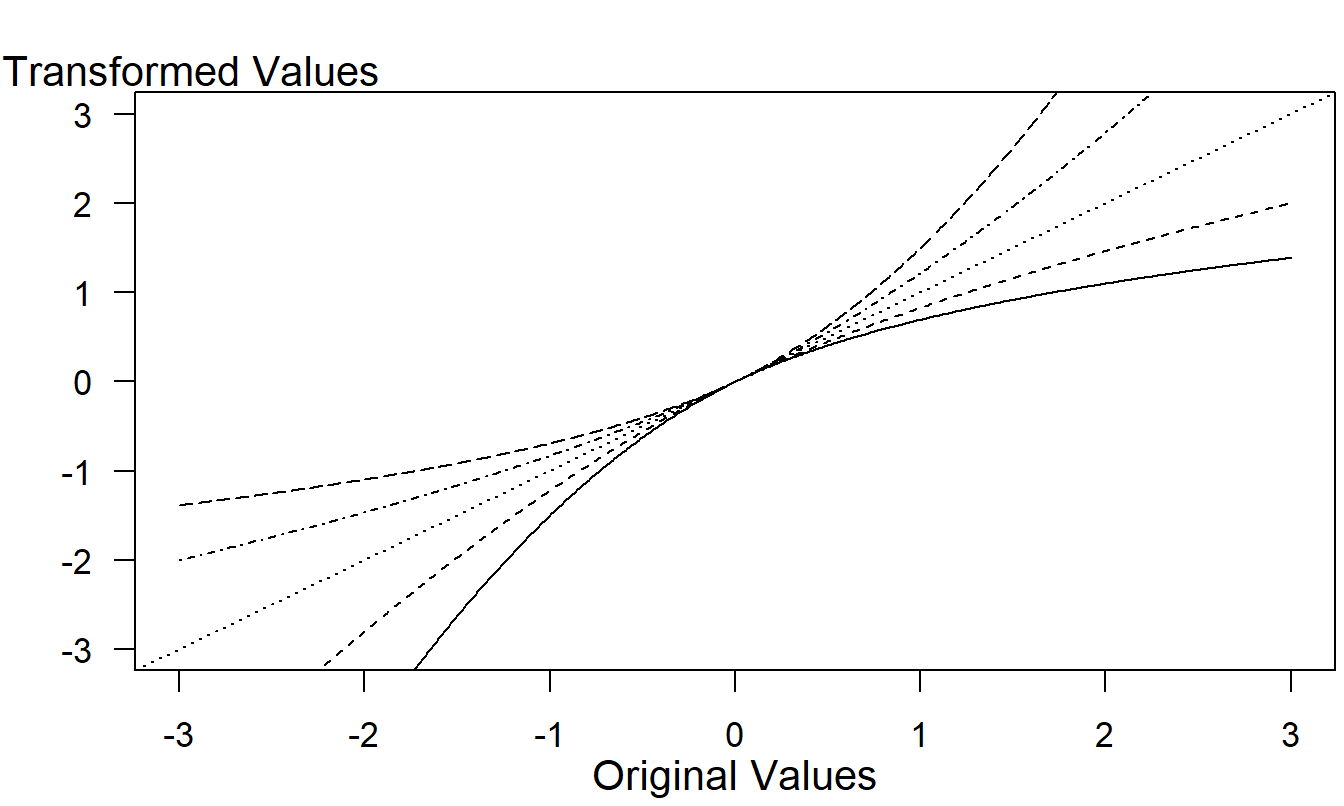
Figure 17.1: Yeo-Johnson Transformations. From bottom to top, the curves correspond to \(\lambda =0,0.5,1,1.5\) and 2.
Both the John and Draper as well as the Yeo and Johnson families are based on power transforms. An alternative family, due to Burbidge and Magee (1988), is a modification of the inverse hyperbolic sine transformation. This family is given by: \[ y^{(\lambda)}=\sinh^{-1}(\lambda y)/\lambda . \]
17.3 Generalized Linear Models
As introduced in Chapter 13, the generalized linear model (GLM) method has become popular in financial and actuarial statistics. An advantage of this methodology is the ability to fit distributions with tails heavier than the normal distribution. In particular, GLM methods are based on the exponential family that includes the normal, gamma and inverse gaussian distributions. As we will see in Section 17.3.1, it is customary to think of the gamma distribution as having intermediate tails and the inverse gaussian as having heavy tails compared to the thin-tailed normal distribution.
The idea of a GLM is to map a linear systematic component \(\mathbf{x}^{\prime }\boldsymbol \beta\) into the mean of the variable of interest through a known function. Thus, GLMs provide a natural way to include covariates into the modeling. With a GLM, the variance is not required to be constant as in the linear model, but is a function of the mean. Once the distribution family and link function have been specified, estimation of GLM regression coefficients depends only on the mean and thus is robust to some model distribution mis-specifications. This is both a strength and weakness of the GLM approach. Although more flexible than the linear model, this approach does not handle many of the long-tail distributions traditionally used for modeling insurance data. Thus, in Section 17.4 we will present more flexible distributions.
17.3.1 What is “Fat-Tailed?”
Many analysts begin discussions of tail heaviness through skewness and kurtosis coefficients. Skewness measures the lack of symmetry, or lop-sidedness, of a distribution. It is typically quantified by the third standardized moment, \(\mathrm{E}(y-\mathrm{E~}y)^3/ (\mathrm{Var~}y)^{3/2}.\) Kurtosis measures tail heaviness, or its converse, “peakedness.” It is typically quantified by the fourth standardized moment minus 3, \(\mathrm{E}(y-\mathrm{E~}y)^4/ (\mathrm{Var~}y)^{2} -3.\) The “minus 3” is to center discussions around the normal distribution; that is, for a normal distribution, one can check that \(\mathrm{E}(y-\mathrm{E~}y)^4/(\mathrm{Var~}y)^{2} =3.\) Distributions with positive kurtosis are called leptokurtic whereas those with negative kurtosis are called platykurtic. These definitions focus heavily on the normal that has traditionally been viewed as the benchmark distribution.
For many actuarial and financial applications, the normal distribution is not an appropriate starting point and so we seek other definitions of “fat-tail.” In addition to moments, the size of the tail can be measured using a density (or mass, for discrete distributions) function, the survival function, or a conditional moment. Typically, the measure would be used to compare one distribution to another.
For example, comparing the right tails of the normal to a gamma density function, we have \[ \begin{array}{ll} \frac{\mathrm{f}_{normal}\left( y\right) }{\mathrm{f}_{gamma}\left( y\right) } &=\frac{\sqrt{2\pi \sigma ^{2}}\exp \left( -\left( y-\mu \right) ^{2}/(2\sigma ^{2})\right) }{\left[ \lambda ^{\alpha }\Gamma \left( \alpha \right) \right] ^{-1}y^{\alpha -1}\exp \left( -y/\lambda \right) } \\ &=C_1 ~\mathit{\exp }\left( -(\alpha -1)\ln y+y/\lambda -\left( y-\mu \right) /(2\sigma ^{2})\right) \\ &\rightarrow 0, \end{array} \] as \(y \rightarrow \infty\), indicating that the gamma has a heavier, or fatter, tail than the normal.
Both the normal and the gamma are members of the exponential family of distributions. For comparison with another member of this family, the inverse gaussian distribution, consider \[ \begin{array}{ll} \frac{\mathrm{f}_{gamma}\left( y\right) }{\mathrm{f}_{invGaussian}\left( y\right) } &=\frac{\left[ \lambda ^{\alpha }\Gamma \left( \alpha \right) \right] ^{-1}y^{\alpha -1}\exp \left( -y/\lambda \right) }{\sqrt{\theta /(2\pi y^{3})}\exp \left( -\theta \left( y-\mu \right) ^{2}/(2y\mu ^{2})\right) } \\ &=C_2 ~\mathit{\exp }\left( (\alpha +1/2)\ln y-y/\lambda +\theta \left( y-\mu \right) ^{2}/(2y\mu ^{2}))\right) . \end{array} \] As \(y\rightarrow \infty\), this ratio tends to zero for \(\theta /(2\mu ^{2})<\lambda\), indicating that the inverse gaussian can have a heavier tail than the gamma.
For a distribution that is not a member of the exponential family, consider the Pareto distribution. Similar calculations show \[ \begin{array}{ll} \frac{\mathrm{f}_{gamma}\left( y\right) }{\mathrm{f}_{Pareto}\left( y\right) } &=\frac{\left[ \lambda ^{\alpha }\Gamma \left( \alpha \right) \right] ^{-1}y^{\alpha -1}\exp \left( -y/\lambda \right) }{\alpha \theta ^{-\alpha }\left( y+\theta \right) ^{-\alpha -1}} \\ &=C_3 ~\mathit{\exp }\left( (\alpha -1)\ln y-y/\lambda +\left( \alpha +1\right) \ln \left( y+\theta \right) \right) \\ & \rightarrow 0, \end{array} \] as \(y\rightarrow \infty\), indicating that the Pareto has a heavier tail than the gamma.
The ratio of densities is an easily interpretable measure for comparing the tail heaviness of two distributions. Because densities and survival functions have a limiting value of zero, by L’Höpital’s rule the ratio of survival functions is equivalent to the ratio of densities. That is, \[ \lim_{y\rightarrow \infty }\frac{\mathrm{S}_1\left( y\right) }{\mathrm{S} _2\left( y\right) }=\lim_{y\rightarrow \infty }\frac{\mathrm{S} _1^{\prime }\left( y\right) }{\mathrm{S}_2^{\prime }\left( y\right) } = \lim_{y\rightarrow \infty }\frac{\mathrm{f}_1 \left( y\right) }{\mathrm{f}_2 \left( y\right) }. \] This provides another motivation for using this measure.
17.3.2 Application: Wisconsin Nursing Homes
Nursing home financing has drawn the attention of policymakers and researchers for the past several decades. With aging populations and increasing life expectancies, expenditures on nursing homes and demands of long term care are expected to increase in the future. In this section, we analyze the data of 349 nursing facilities in the State of Wisconsin in the cost report year 2001.
The state of Wisconsin Medicaid program funds nursing home care for individuals qualifying on the basis of need and financial status. Most, but not all, nursing homes in Wisconsin are certified to provide Medicaid-funded care. Those that do not accept Medicaid are generally paid directly by the resident or the resident’s insurer.
Similarly, most, but not all, nursing facilities are certified to provide Medicare-funded care. Medicare provides post-acute care for 100 days following a related hospitalization. Medicare does not fund care provided by intermediate care facilities to individuals with developmental disabilities. As part of the conditions for participation, Medicare-certified nursing homes must file an annual cost report to the Wisconsin Department of Health and Family Services summarizing the volume and cost of care provided to all of its residents, Medicare-funded and otherwise.
Nursing homes are owned and operated by a variety of entities, including the state, counties, municipalities, for-profit businesses and tax-exempt organizations. Private firms often own several nursing homes. Periodically, facilities may change ownership and, less frequently, ownership type.
Typically, utilization of nursing home care is measured in patient days. Facilities bill the fiscal intermediary at the end of each month for total patient days incurred in the month, itemized by resident and level of care. Projections of patient days by facility and level of care play a key role in the annual process of updating facility rate schedules. Rosenberg et al. (2007) provides additional discussion.
Summarizing the Data
After examining the data, we found some minor variations in the number of days that a facility was open, primarily due to openings and closing of facilities. Thus, to make utilization more comparable among facilities, we examine TPY, defined to be the total number of patient days divided by the number of days the facility was open; this has a median value of 81.99 per facility.
Table 17.1 describes the variables that will be used to explain the distribution of TPY. More than half of the facilities have self funding of insurance. Approximately \(90.5\%\) of the facilities are Medicare Certified. Regarding the organizational structure, about half \((51.9\%)\) are run on a for-profit basis, and about one third \((37.5\%)\) are organized as tax exempt and the remainder are governmental organizations. The tax exempt facilities have the highest median occupancy rates. Slightly more than half of the facilities are located in an urban environment (53.3%).
| Variable | Description | ||
|---|---|---|---|
| TPY | Total person years (median 81.89) | ||
| NumBed | Number of beds (median 90) | ||
| SqrFoot | Nursing home net square footage (in thousands, median 40.25) | ||
| Categorical Explanatory Variables | Percentage | Median TPY | |
| POPID | Nursing home identification number | ||
| SelfIns | Self Funding of Insurance | ||
| Yes | 62.8 | 88.4 | |
| No | 37.2 | 67.84 | |
| MCert | Medicare Certified | ||
| Yes | 90.5 | 84.06 | |
| No | 9.5 | 53.38 | |
| Organizational | Pro (for profit) | 51.9 | 77.23 |
| Structure | TaxExempt (tax exempt) | 37.5 | 81.13 |
| Govt (governmental unit) | 10.6 | 106.7 | |
| Location | Urban | 53.3 | 91.55 |
| Rural | 46.7 | 74.12 |
Fitting Generalized Linear Models
Figure 17.2 shows the distribution of the dependent variable TPY. From this figure, we see clear evidence of the right-skewness of the distribution. One option would be to take a transform as described in Section 17.2. Rosenberg et al. (2007) explored this option using a logarithmic transformation.
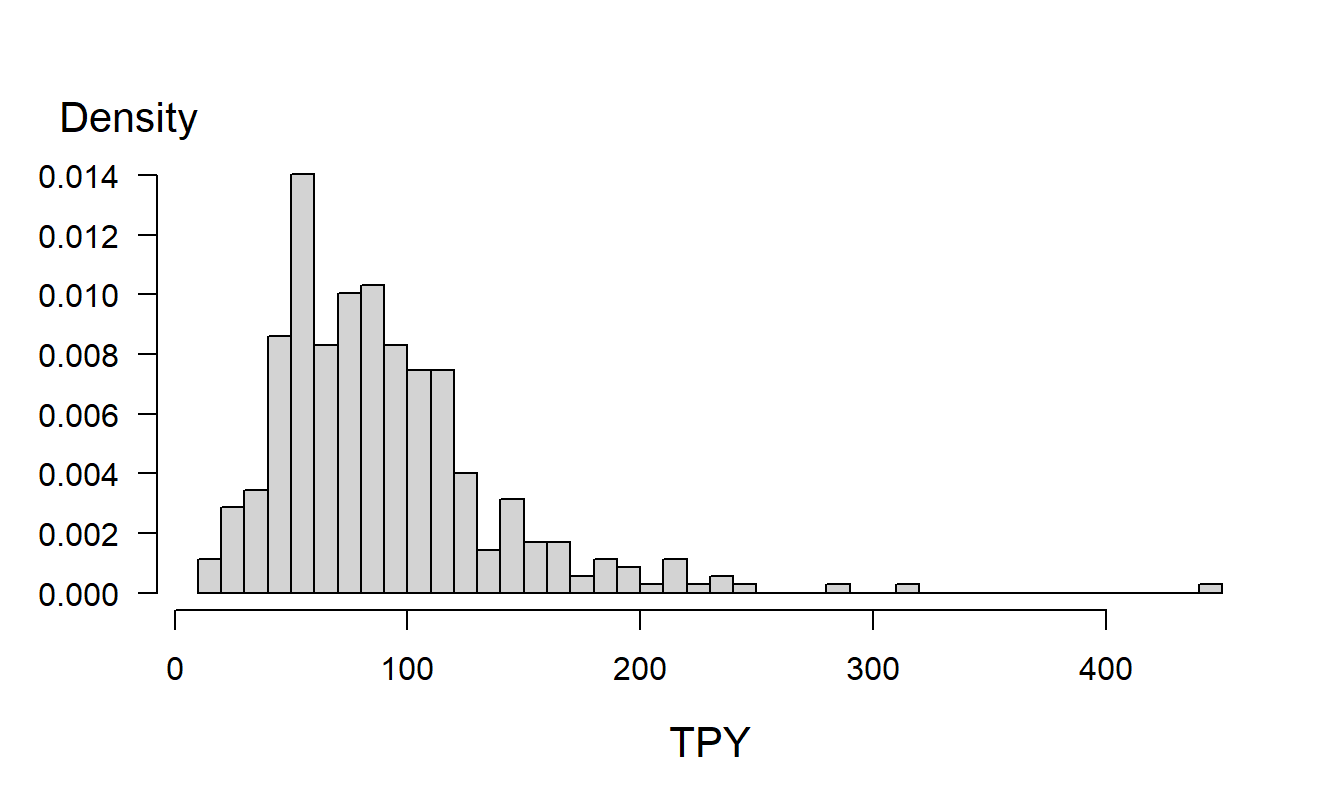
Figure 17.2: Histogram of TPY. This plot demonstrates the right skewness of the distribution.
R Code to Produce Figure 17.2
Another option is to directly fit a skewed distribution to the data. Figure 17.3 presents the \(qq\) plots of the gamma and inverse gaussian distributions. The data fall fairly close to the line in both panels, meaning both models are reasonable choices. The normal \(qq\) plot, not shown here, indicates that the normal regression model is not a reasonable fit.
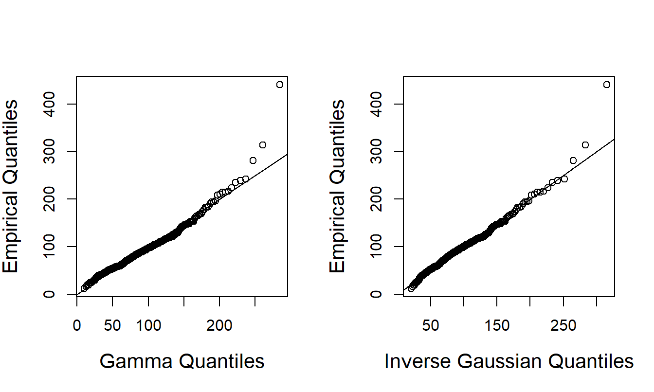
Figure 17.3: \(qq\) Plots of TPY for the Gamma and Inverse Gaussian Distributions
R Code to Produce Figure 17.3
We fit the generalized linear models using the gamma and inverse gaussian distributions. In both models, we choose the logarithmic link function. The linear systematic component that is common to each model is \[\begin{eqnarray} && \eta = \beta_0 + \beta_1 \ln(\text{NumBed}) + \beta_2 \ln(\text{SqrFoot}) + \beta_3 \text{Pro} \\ && + \beta_4 \text{TaxExempt} + \beta_5 \text{SelfIns} + \beta_6 \text{MCert} + \beta_7 \text{Urban}. \notag \tag{17.1} \end{eqnarray}\]
Table 17.2 summarizes the parameter estimates of the models. By comparing the BIC statistics, or the AIC and log-likelihood in that the number of estimated parameters and the sample size in both models are identical, we find the gamma model performs better than the inverse gaussian. As anticipated, the coefficient for the size variable NumBed is positive and significant. The only other variable that is statistically significant is the SqrFoot variable, and this only in the gamma model.
Table 17.2. Fitted Nursing Home Generalized Linear Models
\[ \small{ \begin{array}{l|rr|rr} \hline\hline &\text{Gamma} & & \text{Inverse} & \text{Gaussian} \\ \text{Variables} & \text{Estimate} & \textit{t}\text{-ratio} & \text{Estimate} & \textit{t}\text{-ratio}\\ \hline \text{Intercept} & -0.159 & -3.75 & -0.196 & -4.42 \\ \text{ln(NumBed) } & 0.996 & 66.46 & 1.023 & 65.08 \\ \text{ln(SqrFoot)} & 0.026 & 2.07 & 0.003 & 0.19 \\ \text{SelfIns} & 0.006 & 0.75 & 0.003 & 0.27 \\ \text{MCert } & -0.008 & -0.55 & -0.008 & -0.57 \\ \text{Pro} & 0.004 & 0.29 & 0.007 & 0.36 \\ \text{TaxExempt} & 0.018 & 1.28 & 0.021 & 1.12 \\ \text{Urban} & -0.011 & -1.25 & -0.006 & -0.64 \\ \text{Scale} & 165.64& & 0.0112 \\ \hline \\ \hline \end{array} \\ \text{Goodness of Fit Statistics} \\ \begin{array}{lrr} \hline \text{Log Likelihood} & -1,131.24 & -1,218.15 \\ \text{AIC} &2,280.47 & 2,454.31\\ \text{BIC} & 2,315.17 & 2,489.00 \\ \hline\hline \end{array} } \]
Figure 17.4 presents the plots of deviance residuals against the fitted value of TPY for the gamma and inverse gaussian models. No patterns are found in the plots, supporting the position that these models are reasonable fits to the data.
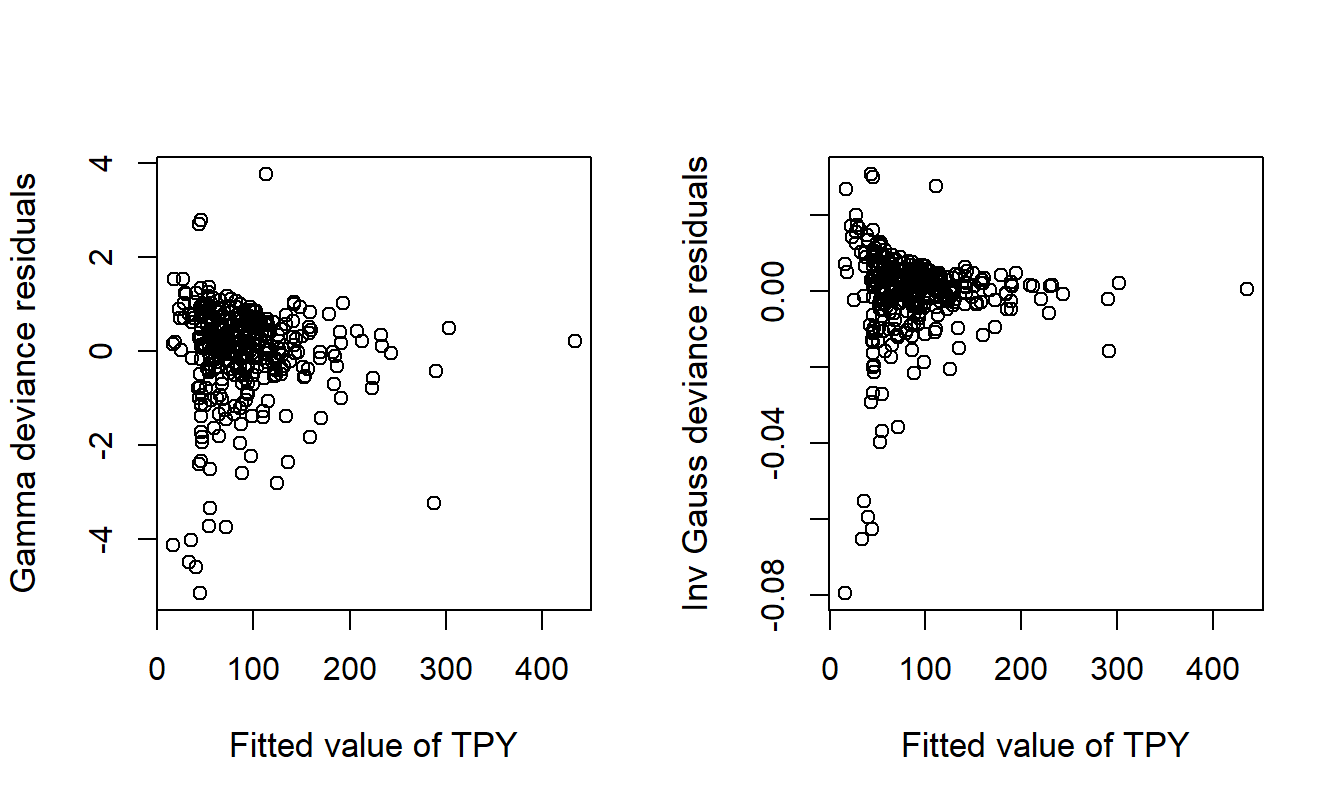
Figure 17.4: Plots of Deviance Residuals versus Fitted Values for the Gamma and Inverse Gaussian Models.
R Code to Produce Figure 17.4
17.4 Generalized Distributions
Another approach for handling fat-tailed regression data is to use parametric distributions, such as those from the survival modeling. Although survival analysis focuses on censored data, the methods can certainly be applied to complete data. In Section 14.3 we introduced an accelerated failure time (AFT) model. The AFT is a log location-scale model, so that \(\ln (y)\) follows a parametric location-scale density distribution in the form \(\mathrm{f}(y)=\mathrm{f}_0\left( (y-\mu )/\sigma \right) /\sigma\), where \(\mu\) and \(\sigma >0\) are location and scale parameters, and \(\mathrm{f}_0\) is the standard form of the distribution. The Weibull, lognormal and loglogistic distributions are commonly used lifetime distributions that are special cases of the AFT framework.
For fitting fat-tailed distributions of interest in actuarial science, we consider the following minor variation, and examine distributions from the relation \[\begin{equation} \ln y = \mu + \sigma \ln y_0. \tag{17.2} \end{equation}\] As before, the distribution associated with \(y_0\) is a standard one and we are interested in the distribution of the random variable \(y\). Two important special cases are the generalized gamma and the generalized beta of the second kind. These distributions have been used extensively in modeling insurance data, see for example, Klugman et al. (2008), although most applications have not utilized regression covariates.
The generalized gamma distribution is obtained when \(y_0\) has a gamma distribution with shape parameter \(\alpha\) and scale parameter 1. When including limiting distributions (such as allowing coefficients to become arbitrarily large), it includes the exponential, Weibull, gamma, and lognormal distributions as special cases. Therefore, it can be used to discriminate between the alternate models. The generalized gamma distribution is also known as the transformed gamma distribution (Klugman et al., 2008).
When \(y_0\) has a distribution that is the ratio of two gammas, then \(y\) is said to have a generalized beta of the second kind distribution, commonly known by the acronym GB2. Specifically, we assume that \(y_0 = Gamma_1/Gamma_2\), where \(Gamma_i\) has a gamma distribution with shape parameter \(\alpha_i\) and scale parameter 1, \(i=1,2\), and that \(Gamma_1\) and \(Gamma_2\) are independent. Thus, the GB2 family has four parameters (\(\alpha_1\), \(\alpha_2\), \(\mu\) and \(\sigma\)) compared to the three parameter generalized gamma distribution. When including limiting distributions, the GB2 encompasses the generalized gamma (by allowing \(\alpha_2 \rightarrow \infty)\) and hence the exponential, Weibull, and so forth. It also encompasses the Burr Type 12 (by allowing \(\alpha_1 = 1\)), as well as other families of interest, including the Pareto distributions.
The distribution of \(y\) from equation (17.2) contains location parameter \(\mu\), scale parameter \(\sigma\) and additional parameters that describe the distribution of \(y_0\). In principle, one could allow for any distribution parameter to be a function of the covariates. However, following this principle would lead to a large number of parameters; this typically yields computational difficulties as well as problems of interpretations. To limit the number of parameters, it is customary to assume that the parameters from \(y_0\) do not depend on covariates. It is natural to allow the location parameter to be a linear function of covariates so that \(\mu =\mu \left( \mathbf{x}\right)= \mathbf{x}^{\prime } \boldsymbol \beta\). One may also allow the scale parameter \(\sigma\) to depend on \(\mathbf{x}\). For \(\sigma\) positive, a common specification is \(\sigma =\sigma (\mathbf{x})\) \(= \exp(\mathbf{x}^{\prime }\boldsymbol \beta_{\sigma })\), where \(\boldsymbol \beta_{\sigma}\) are regression coefficients associated with the scale parameter. Other parameters are typically held fixed.
The interpretability of parameters is one reason to hold the scale and other non-location parameters fixed. By doing this, it is straightforward to show that the regression function is of the form \[ \mathrm{E}\left( y|\mathbf{x}\right) =C\exp \left( \mu \left( \mathbf{x} \right) \right) =C~e^{\mathbf{x}^{\prime }\boldsymbol \beta}, \] where the constant \(C\) is a function of other (non-location) model parameters. Thus, one can interpret the regression coefficients in terms of a proportional change (an elasticity in economics). That is, \(\partial \left[ \ln \mathrm{E}(y) \right] /\partial x_k= \beta_k.\)
Another reason for holding non-location parameters fixed is the ease of computing sensible residuals and using these residuals to assist with model selection. Specifically, with equation (17.2), one can compute residuals of the form \[ r_i = \frac{\ln y_i-\widehat{\mu}_i }{\widehat{\sigma }}, \] where \(\widehat{\mu}_i\) and \(\widehat{\sigma }\) are maximum likelihood estimates. For large data sets, we may assume little estimation error so that \(r_i \approx (\ln y_i - \mu_i) /\sigma,\) and the quantity on the right-hand side has a known distribution.
To illustrate, consider the case when \(y\) follows a GB2 distribution. In this case, \[ y_0 = \frac{Gamma_1}{Gamma_2}= \frac{\alpha_1}{\alpha_2} \times \frac{Gamma_1/(2\alpha_1)}{Gamma_2/(2\alpha_2)} = \frac{\alpha_1}{\alpha_2} \times F , \] where \(F\) has an \(F\)-distribution with numerator and denominator degrees of freedom \(df_1 = 2 \alpha_1\) and \(df_2 = 2 \alpha_2\). Then, \(\exp(r_i) \approx (\alpha_1 /\alpha_2) F_i\), so that the exponentiated residuals should have an approximate F-distribution (up to a scale parameter). This fact allows us to compute quantile-quantile (qq) plots to assess model adequacy graphically.
To illustrate, we consider a few insurance related examples that use fat-tailed regression models. McDonald and Butler (1990) discussed regression models including those commonly used as well as the GB2 and generalized gamma distribution. They applied the model to the duration of poverty spells and found that the GB2 improved model fitting significantly over the lognormal. Beirlant et al. (1998) proposed two Burr regression models, and applied them to portfolio segmentation for fire insurance. The Burr is a an extension of the Pareto distribution, although still a special case of the GB2. Manning, Basu and Mullahy (2005) applied the generalized gamma distribution to inpatient expenditures using the data from a study of hospitals conducted at the University of Chicago.
Because the regression model is fully parametric, maximum likelihood is generally the estimation method of choice. If \(y\) follows a GB2 distribution, straight-forward calculations show that its density can be expressed as \[\begin{equation} f(y; \mu, \sigma, \alpha_1, \alpha_2) = \frac{[\exp( z)]^{\alpha_{1}}}{y |\sigma| B(\alpha_1, \alpha_2) [1 + \exp(z) ]^{\alpha_1 + \alpha_2} }, \tag{17.3} \end{equation}\] where \(z= (\ln y - \mu)/{\sigma}\) and B(\(\cdot,\cdot\)) is the beta function, defined as \(\text{B}(\alpha_1, \alpha_2) = \Gamma(\alpha_1)\Gamma(\alpha_2)/\Gamma(\alpha_1+\alpha_2)\). This density can be used directly in likelihood routines of many statistical packages. As described in Section 11.9, the method of maximum likelihood automatically provides:
- standard errors for the parameter estimates,
- methods of model selection via likelihood ratio testing and
- goodness of fit statistics such as AIC and BIC.
Application: Wisconsin Nursing Homes
In the fitted generalized linear models summarized in Table Table 17.2, we saw that the coefficients associated with ln(NumBed) were close to one. This suggest identifying ln(NumBed) as an offset variable, that is, forcing the coefficient associated with ln(NumBed) to be 1. For another modeling strategy, it also suggests rescaling the dependent variable by NumBed. This is sensible because we used a logarithmic link function so that the expected value of TPY is proportional to NumBed. Pursuing this approach, we now define the annual occupancy rate (Rate) to be \[\begin{equation} \text{Occupancy Rate} = \frac{\text{Total Patient Days}}{\text{Number of Beds} \times \text{Days Open}} \times 100. \tag{17.4} \end{equation}\] This new dependent variable is easy to interpret - it measures the percentage of beds being used on any given day. Occupancy rates were calculated using the average number of licensed beds within a cost report year rather than the number of licensed beds on a specific day. This gives rise to a few occupancy rates greater than 100.
One difficulty of using occupancy rates is that its distribution cannot reasonably be approximated by a member of the exponential family. Figure 17.5 shows a smoothed histogram of the Rate variable (using a kernel smoother); this distribution is left-skewed. Superimposed on it with the dotted line is the inverse gaussian distribution where the parameters were fit without covariates, using method of moments. The gamma and normal distributions are very close to the inverse gaussian, and hence are not shown here. In contrast, the fitted (also without covariates) GB2 distribution shown in Figure 17.5 captures important parts of the distribution; in particular, it captures the peakedness and left-skewness.
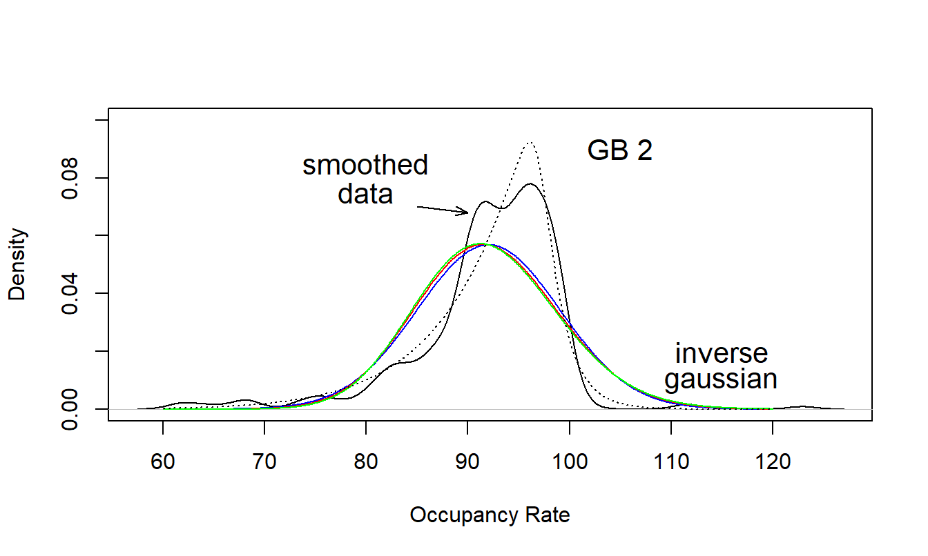
Figure 17.5: Nursing Home Densities. The empirical version, based on a kernel density estimate, is compared to fitted GB2 and inverse gaussian densities.
R Code to Produce Figure 17.5
The GB2 distribution was fit using maximum likelihood with the same covariates as in Table 17.2. Specifically, we used location parameter \(\mu = \exp(\eta)\), where \(\eta\) is specified in equation (17.1). As is customary in likelihood estimation, we reparameterized the scale and two shape parameters, \(\sigma\), \(\alpha_1\) and \(\alpha_2\), to be transformed on the log scale so that they could range over the whole real line. In this way, we avoided boundary problems that could arise when trying to fit models with negative parameter values. Table 17.3 summarizes the fitted model. Unfortunately, for this fitted model, none of the explanatory variables turned out to be statistically significant. (Recall that we rescaled by number of beds, a very important explanatory variable.)
Table 17.3. Wisconsin Nursing Home Generalized Models Fits
\[ \small{ \begin{array}{l|rr|rr} \hline \hline \hline & \text{Generalized }& \text{Gamma} &\text{GB2} \\ \hline \text{Variables} & \text{Estimate} & \textit{t}\text{-ratio} &\text{Estimate} & \textit{t}\text{-ratio} \\ \hline \text{Intercept} & 4.522 & 78.15 & 4.584 & 198.47 \\ \text{ln(NumBed)} & -0.027 & -2.06 & -0.010 & -1.17 \\ \text{ln(SqrFoot)} & 0.031 & 2.89 & 0.010 & 1.28 \\ \text{SelfIns} & 0.003 & 0.44 & -0.001 & -0.25 \\ \text{MCert} & -0.010 & -0.81 & -0.010 & -1.30 \\ \text{Pro } & -0.021 & -1.46 & -0.002 & -0.20 \\ \text{TaxExempt} & -0.007 & -0.48 & 0.015 & 1.66 \\ \text{Urban} & -0.014 & -1.78 & -0.003 & -0.60 \\ \hline & \text{Estimate} &\text{Std Error} & \text{Estimate} & \text{Std Error} \\ \ln \sigma & -2.406 & 0.131 & -5.553 & 1.716 \\ \ln \alpha_1 & 0.655 & 0.236 & -2.906 & 1.752 \\ \ln \alpha_2 & & & -1.696 & 1.750 \\ \end{array} \\ \begin{array}{l|rr} \hline \text{Log-Likelihood} &-1,148.135 & -1,098.723 \\ \text{AIC} & 2,316.270 & 2,219.446 \\ \text{BIC} & 2,319.296 & 2,223.822\\ \hline\hline \end{array} } \]
To further assess the model fit, Figure 17.6 shows residuals from this fitted model. For these figures, residuals are computed using \(r_i = (\ln y_i-\widehat{\mu}_i)/\widehat{\sigma }.\) The left-hand panel shows the residuals versus fitted values (\(\exp(\widehat{\mu}_i)\)), no apparent patterns are evident in this display. The right-hand panel is a \(qq\) plot of residuals, where the reference distributions is the logarithmic \(F\)-distribution (plus a constant) described above. This figure shows some discrepancies for smaller values of nursing homes. Because of this, Table 17.3 also reports fits from the generalized gamma model. This fit is more pleasing in the sense that two of the explanatory variable are statistically significant. However, from the goodness of fit statistics, we see that the GB2 is a better fitting model. Note that the goodness of fit statistics for the generalized gamma model are not directly comparable with the gamma regression fits in Table 17.2; this is only because the dependent variable differs by the scale variable NumBeds.
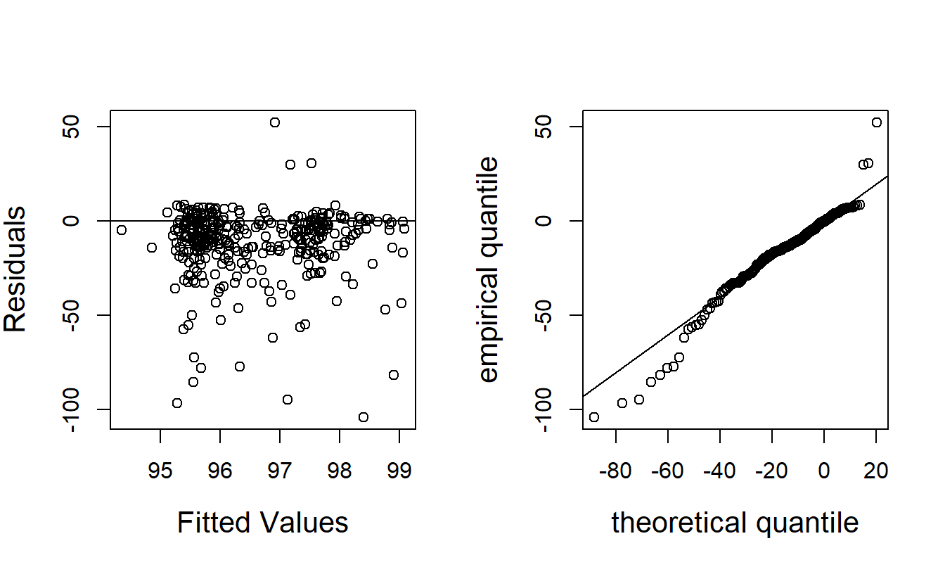
Figure 17.6: Residual Analysis of the GB2 Model. The left-hand panel is a plot of residuals versus fitted values. The right-hand panel is a \(qq\) plot of residuals.
R Code to Produce Figure 17.6
17.5 Quantile Regression
Quantile regression is an extension of median regression, so it is helpful to introduce this concept first.
In median regression, one finds the set of regression coefficients \(\boldsymbol \beta\) that minimizes
\[ \sum_{i=1}^n | y_i - \mathbf{x}_i^{\prime} \boldsymbol \beta |. \] That is, we simply replace the usual squared loss function with an absolute value function. Although we will not go into the details here, finding these optimal coefficients is a simple optimization problem in nonlinear programming that can be readily implemented in modern statistical software.
Because this procedure uses the absolute value as the loss function, median regression is also known as LAD for least absolution deviations as compared to OLS (for ordinary least squares). The adjective “median” comes from the special case where there are no regressors so that \(\mathbf{x}\) is a scalar 1. In this case the minimization problem reduces to finding an intercept \(\beta_0\) that minimizes
\[ \sum_{i=1}^n | y_i - \beta_0 |. \] The solution to this problem is the median of \(\{y_1, \ldots, y_n\}\).
Suppose that you would also like to find the \(25^{th}\), \(75^{th}\), or some other percentile of \(\{y_1, \ldots, y_n\}\). One can also use this optimization procedure to find any percentile, or quantile. Let \(\tau\) be a fraction between 0 and 1. Then, the \(\tau\)th sample quantile of \(\{y_1, \ldots, y_n\}\) is the value of \(\beta_0\) that minimizes \[ \sum_{i=1}^n \rho_{\tau}( y_i - \beta_0). \] Here, \(\rho_{\tau}(u)=u(\tau-{\rm I}(u\leq0))\) is called a check function and \({\rm I}(\cdot)\) is the indicator function.
Extending this procedure, in quantile regression one finds the set of regression coefficients \(\boldsymbol \beta\) that minimizes \[ \sum_{i=1}^n \rho_{\tau}( y_i - \mathbf{x}_i^{\prime} \boldsymbol \beta ). \] The estimated regression coefficients depend on the fraction \(\tau\), so we use the notation \(\widehat{\boldsymbol \beta}(\tau)\) to emphasize this dependence. The quantity \(\mathbf{x}_i^{\prime}\widehat{\boldsymbol \beta}(\tau)\) represents the \(\tau^{\rm th}\) quantile of the distribution of \(y_i\) for the explanatory vector \(\mathbf{x}_i\). To illustrate, for \(\tau = 0.5\), \(\mathbf{x}_i^{\prime}\widehat{\boldsymbol \beta}(0.5)\) represents the estimated median of the distribution of \(y_i\). In contrast, the \(OLS\) fitted value \(\mathbf{x}_i^{\prime}\mathbf{b}\) represents the estimated mean of the distribution of \(y_i\).
Example: Wisconsin Nursing Homes - Continued. To illustrate quantile regression techniques, we fit a regression of square footage (SqrFoot) on total person years (TPY). Figure 17.7 shows the relationship between these two variables, with mean (OLS) and median (LAD) fitted lines superimposed. Unlike the original TPY distribution that is skewed, for each value of SqrFoot we can see little difference between the mean and median values. This suggests that the conditional distribution of TPY given SqrFoot is not skewed.
Figure 17.7 also shows the fitted lines that result from fitting quantile regressions at four additional values of \(\tau =0.05,0.25, 0.75\) and 0.95. These fits are indicated by the grey lines. At each value of SqrFoot, we can visually get a sense of the \(5^{th}\), \(25^{th}\), \(50^{th}\), \(75^{th}\), and \(95^{th}\) percentiles of the distribution of TPY. Although classic ordinary least squares also provides this, the classic recipes generally assume homoscedasticity. From 17.7, we see that the distribution of \(y\) seems to widen as SqrFoot increases, suggesting a heteroscedastic relationship.
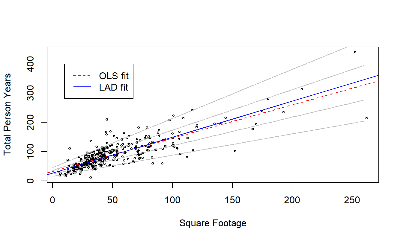
Figure 17.7: Quantile Regression Fits of Square Footage on Total Person Years. Superimposed are fits from mean (OLS) and median (LAD) regressions, indicated in the legend. Also superimposed with grey lines are quantile regression fits – from bottom to top, the fits correspond to \(\tau =0.05,0.25, 0.75\) and 0.95.
R Code to Produce Figure 17.7
Quantile regressions perform well in situations when ordinary least squares requires careful attention to be used with confidence. As demonstrated in the Wisconsin Nursing Home example, quantile regression handles skewed distributions and heteroscedasticity readily. Just as ordinary quantiles are relatively robust to unusual observations, quantile regression estimates are much less sensitive to outlying observations than the usual regression routines.
17.6 Extreme Value Models
Extreme value models focus on the extremes, the “tip of the iceberg,” such as the highest temperature over a month, the fastest time to run a kilometer or the lowest return from the stock market. Some extreme value models are motivated by maximal statistics. Suppose that we consider annual chief executive officer (CEO) compensation in a country, \(y_1, y_2, \ldots\). Then, \(M = \max(y_1, \ldots, y_n)\) represents the compensation of the most highly paid CEO during the year. If values \(y\) were observed, then we could use some mild additional assumptions (such as independence) to make inference about the the distribution of \(M\). However, in many cases, only \(M\) is directly observed, forcing us to base inference procedures on “extreme” observations \(M\). As a variation, we might have observations for the top 20 CEO’s – not the entire population. This variation uses inference based on the “20” largest order statistics, see for example Coles (2003, Section 3.5.2).
Modeling \(M\) is often based on the generalized extreme value, or \(GEV\), distribution, defined by the distribution function \[\begin{equation} \Pr(M \leq x) = \exp \left[-(1+ \gamma z )^{-1/\gamma} \right], \tag{17.5} \end{equation}\] where \(z=(x-\mu)/ \sigma\). This is a location-scale model, with location and scale parameters \(\mu\) and \(\sigma\), respectively. In the standard case where \(\mu=0\) and \(\sigma=1\), allowing \(\gamma \rightarrow \infty\) means that \(\Pr(M \leq x) \rightarrow \exp \left[- e^{-x} \right],\) the classical extreme value distribution. Thus, the parameter \(\gamma\) provides the generalization of this classical distribution.
Beirlant, Goegebeur, Segers and Teugels (2004) discuss ways in which one could introduce regression covariates into the \(GEV\) distribution, essentially by allowing each parameter to depend on covariates. Estimation is done via maximum likelihood. In their inference procedures, the focus is on the behavior of the extreme quantiles (conditional on the covariates).
Another approach to modeling extreme values is to focus on data that must be large to be included in the sample.
Example: Large Medical Claims. Cebrián, Denuit and Lambert (2003) analyzed 75,789 large group medical insurance claims from 1991. To be included in this database, claims must exceed 25,000. Thus, these data are left-truncated at 25,000. The interest in their study was to interpret the long-tailed distribution in terms of covariates age and sex.
The peaks over threshold approach to modeling extremes values is motivated by left-truncated data where the truncation point, or “threshold,” is large. To be included in the data set, the observations must exceed a large threshold that we refer to as a “peak.” Following our Section 14.2 discussion on truncation, if \(C_L\) is the left truncation point, then the distribution function of \(y-C_L\) given that \(y>C_L\) is \(1 - \Pr(y-C_L > x |y>C_L)\) \(= 1 - (1-F_y(C_L+x))/(1-F_y(C_L))\). Instead of modeling the distribution of \(y\), \(F_y\), directly as in prior sections, one assumes that it can be directly approximated by a generalized Pareto distribution. That is, we assume \[\begin{equation} \Pr(y-C_L \leq x |y>C_L) \approx 1 - (1+ \frac{z}{\theta} )^{-\theta} , \tag{17.6} \end{equation}\] where \(z=x / \sigma\), \(\sigma\) is a scale parameter, \(x \geq 0\) if \(\theta \geq 0\) and \(0 \leq x \leq - \theta\) if \(\theta < 0\). Here, the right-hand side of equation (17.6) is the generalized Pareto distribution. The usual Pareto distribution restricts \(\theta\) to be positive; this specification allows for negative values of \(\theta\). Allowing \(\theta \rightarrow 0\) means that \(1 - (1+ z/\theta )^{-\theta} \rightarrow 1 - e^{-x/\sigma},\) the exponential distribution.
Example: Large Medical Claims - Continued. To incorporate age and sex covariates, Cebrián et al. (2003) categorized the variables, allowed parameters to vary by category and estimated each category in isolation of the others. Alternative, more efficient, approaches are described in Chapter 7 of Beirlant et al. (2004).
17.7 Further Reading and References
The literature on long-tailed claims modeling is actively developing. A standard reference is Klugman et al (2008). Kleiber and Kotz (2003) provide an excellent survey of the univariate literature, with many historical references. Carroll and Ruppert (1988) provide extensive discussions of transformations in regression modeling.
This chapter has emphasized the GB2 distribution with its many special cases. Venter (2007) discusses extensions of the generalized linear model, focusing on loss reserving applications. Balasooriya and Low (2008) provide a recent applications to insurance claims modeling, although without any regression covariates. Another approach is to use a skewed elliptical (such as a normal or \(t\)-) distribution. Bali and Theodossiou (2008) provide a recent application, showing how to use such distributions in time series modeling of stock returns.
Koenker (2005) is an excellent book-long introduction to quantile regression. Yu, Lu and Stander (2003) provide an accessible shorter introduction.
Coles (2003) and Beirlant et al. (2004) are two excellent book-long introductions to extreme value statistics.
References
- Balasooriya, Uditha and Chan-Kee Low (2008). Modeling insurance claims with extreme observations: Transformed kernel density and generalized lambda distribution. North American Actuarial Journal 11(2) 129-142.
- Bali, Turan G. and Panayiotis Theodossiou (2008). Risk measurement of alternative distribution functions. Journal of Risk and Insurance 75(2), 411-437.
- Beirlant, Jan, Yuir Goegebeur, Robert Verlaak and Petra Vynckier (1998). Burr regression and portfolio segmentation. Insurance: Mathematics and Economics 23, 231-250.
- Beirlant, Jan, Yuir Goegebeur, Johan Segers and Jozef Teugels (2004). Statistics of Extremes. Wiley, New York.
- Burbidge, J.B. and Magee, L. and Robb, A.L. (1988). Alternative transformations to handle extreme values of the dependent variable. Journal of the American Statistical Association 83, 123-127.
- Carroll, Raymond and David Ruppert (1988). Transformation and Weighting in Regression. Chapman-Hall.
- Cebrián, Ana C., Michel Denuit and Philippe Lambert (2003). Generalized Pareto fit to the Society of Actuaries’ large claims database. North American Actuarial Journal 7 (3), 18-36.
- Coles, Stuart (2003). An Introduction to Statistical Modeling of Extreme Values. Springer, New York.
- Cummins, J. David, Georges Dionne, James B. McDonald and B. Michael Pritchett (1990). Applications of the GB2 family of distributions in modeling insurance loss processes. Insurance: Mathematics and Economics 9, 257-272.
- John, J. A. and Norman R. Draper (1980). An alternative family of transformations. Applied Statistics 29 (2), 190-197.
- Kleiber, Christian and Samuel Kotz (2003). Statistical Size Distributions in Economics and Actuarial Sciences. John Wiley and Sons, New York.
- Klugman, Stuart A, Harry H. Panjer and Gordon E. Willmot (2008). Loss Models: From Data to Decisions. John Wiley & Sons, Hoboken, New Jersey.
- Koenker, Roger (2005). Quantile Regression. Cambridge University Press, New York.
- Manning, William G (1998). The logged dependent variable, heteroscedasticity, and the retransformation problem. Journal of Health Economics 17, 283-295.
- Manning, William G, Anirban Basu and John Mullahy (2005). Generalized modeling approaches to risk adjustment of skewed outcomes data. Journal of Health Economics 24, 465-488.
- McDonald, James B. and Richard J. Butler (1990). Regression models for positive random variables. Journal of Econometrics 43, 227-251.
- Rachev, Svetiozar, T., Christian Menn and Frank Fabozzi (2005). Fat-Tailed and Skewed Asset Return Distributions: Implications for Risk Management, Portfolio Selection, and Option Pricing. Wiley, New York.
- Rosenberg, Marjorie A., Edward W. Frees, Jiafeng Sun, Paul Johnson and James M. Robinson (2007). Predictive modeling with longitudinal data: A case study of Wisconsin nursing homes. North American Actuarial Journal 11(3), 54-69.
- Sun, Jiafeng, Edward W. Frees and Marjorie A. Rosenberg (2008). Heavy-tailed longitudinal data modeling using copulas. Insurance: Mathematics and Economics 42(2), 817-830.
- Venter, Gary (2007). Generalized linear models beyond the exponential family with loss reserve applications. Astin Bulletin: Journal of the International Actuarial Association 37 (2), 345-364.
- Yeo, In-Kwon and Richard A. Johnson (2000). A new family of power transformations to improve normality or symmetry. Biometrika 87, 954-959.
- Yu, Keming, Zudi Lu and Julian Stander (2003). Quantile regression: applications and current research areas. Journal of the Royal Statistical Society Series D (The Statistician) 52 (3), 331-350.
17.8 Exercises
17.1. Quantiles and Simulation. Use equation (17.2) to establish the following distributional relationships that are helpful for calculating quantiles.
Assume that \(y_0 = \alpha_1 F/\alpha_2\) where \(F\) has an \(F\)-distribution with numerator and denominator degrees of freedom \(df_1 = 2 \alpha_1\) and \(df_2 = 2 \alpha_2\). Show that \(y\) has a GB2 distribution.
Assume that \(y_0 = B/(1-B),\) where \(B\) has a beta distribution with parameters \(\alpha_1\) and \(\alpha_2\). Show that \(y\) has a GB2 distribution.
Describe how to use parts (a) and (b) for calculating quantiles.
Describe how to use parts (a) and (b) for simulation.
17.2 Consider a GB2 probability density function given in equation (17.3).
Reparameterize the distribution by defining the new parameter \(\theta =e^{\mu }.\) Show that the density can be expressed as: \[ \mathrm{f}_{GB2}(y;\theta, \sigma ,\alpha _1,\alpha _2)=\frac{\Gamma \left( \alpha _1+\alpha _2\right) }{\Gamma \left( \alpha _1\right) \Gamma \left( \alpha _2\right) }\frac{\left( y/\theta \right) ^{\alpha _2/\sigma }}{\sigma y\left[ 1+\left( y/\theta \right) ^{1/\sigma }\right] ^{\alpha _1+\alpha _2}}, \]
Using part (a), show that \[ \lim_{\alpha _2\rightarrow \infty }\mathrm{f}_{GB2}(y; \theta \alpha _2^{\sigma },\sigma ,\alpha _1,\alpha _2)=\frac{1}{\sigma y\Gamma \left( \alpha _1\right) }\left( y/\theta \right) ^{\alpha _1/\sigma }\exp \left( -\left( y/\theta \right) ^{1/\sigma }\right) =\mathrm{f}_{GG}(y;\theta, \sigma, \alpha _1), \] a generalized gamma density.
Using part (a), show that \[ \mathrm{f}_{GB2}(y;\theta, \sigma, 1, \alpha_2)=\frac{\alpha _2\left( y/\theta \right) ^{\alpha _2/\sigma }}{\sigma y\left[ 1+\left( y/\theta \right) ^{1/\sigma }\right] ^{1+\alpha _2}}=\mathrm{f}_{Burr}(y;\theta, \sigma, \alpha _2), \] a Burr Type 12 density.
17.3 Recall that the density of a gamma distribution with shape parameter \(\alpha\) and scale parameter \(\theta\) has a density given by \(\mathrm{f}(y)=\left[ \theta ^{\alpha }\Gamma \left( \alpha \right) \right] ^{-1}y^{\alpha -1}\exp \left( -y/\theta \right)\) and k\(^{th}\) moment given by \(\mathrm{E} (y^{k})=\theta ^{k}\Gamma \left( \alpha +k\right) /\Gamma \left( \alpha \right)\), for \(k>-\alpha .\)
For the GB2 distribution, show that \[ \mathrm{E}(y)=e^{\mu }\frac{\Gamma \left( \alpha _1+\sigma \right) \Gamma \left( \alpha _2-\sigma \right) }{\Gamma \left( \alpha _1\right) \Gamma \left( \alpha _2\right) }. \]
For the generalized gamma distribution, show that \[ \mathrm{E}(y)=e^{\mu }\Gamma \left( \alpha_1 +\sigma \right) /\Gamma \left( \alpha_1 \right) . \]
Calculate the moments of a Burr Type 12 density.