Chapter 10 Longitudinal and Panel Data Models
Chapter Preview. Longitudinal data, also known as panel data, are composed of a cross-section of subjects that we observe repeatedly over time. Longitudinal data allow us to study cross-sectional and dynamic patterns simultaneously; this chapter describes several techniques for visualizing longitudinal data. Two types of models are introduced, fixed and random effects models. This chapter shows how to estimate fixed effects models using categorical explanatory variables. Estimation for random effects models is deferred to a later chapter; this chapter describes when and how to use these models.
10.1 What are Longitudinal and Panel Data?
In Chapters 1–6 we studied cross-sectional regression techniques that allowed us to predict a dependent variable \(y\) using explanatory variables \(x\). For many problems, the best predictor is a value from the preceding period; the times series methods we studied in Chapters 7–9 use the history of a dependent variable for prediction. For example, an actuary seeking to predict insurance claims for a small business will often find that last year’s claims are the best predictor. However, a limitation of time series methods is that they are based on having available many observations over time (typically 30 or more). When studying annual claims from a business, a long time series is rarely available; either businesses do not have the data or, if they do, it is unreasonable to use the same stochastic model for today’s claims as for those 30 years in the past. We would like a model that allows us to use information about company characteristics, explanatory variables such as industry, number of employees, age and gender composition, and so forth, as well as recent claims history. That is, we need a model that combines cross-sectional regression explanatory variables with time series lagged dependent variables as predictors.
Longitudinal data analysis represents a marriage of regression and time series analysis. Longitudinal data are composed of a cross-section of subjects that we observe repeatedly, over time. Unlike regression data, with longitudinal data we observe subjects over time. By observing a cross-section repeatedly, analysts can make better assessments of regression relationships with a longitudinal data design compared to a regression design. Unlike time series data, with longitudinal data we observe many subjects. By observing time series behavior over many subjects, we can make informed assessments of temporal patterns even when only a short (time) series is available. Time patterns are also known as dynamic. With longitudinal data, we can study cross-sectional and dynamic patterns simultaneously.
The descriptor “panel data” comes from surveys of individuals. In this context, a “panel” is a group of individuals surveyed repeatedly over time. We use the terms “longitudinal data” and “panel data” interchangeably although, for simplicity, we often use only the former term.
As we have seen in our Chapter 6 discussion of omitted variables, any new variable can alter our impressions and models of the relationship between \(y\) and an \(x\). This is also true of lagged dependent variables. The following example demonstrates that the introduction of a lagged dependent variable can dramatically impact a cross-sectional regression relationship.
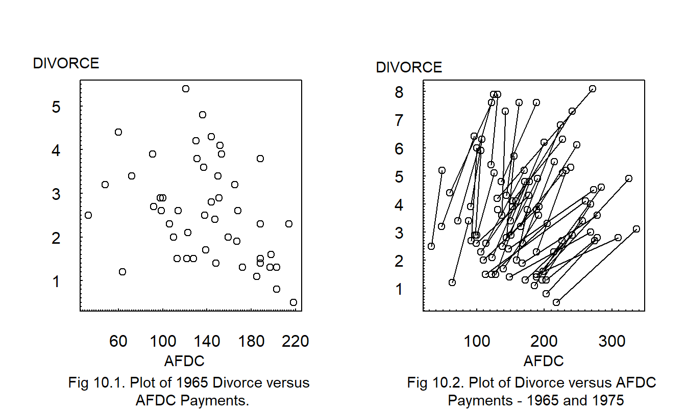
Example: Divorce Rates. Figure 10.1 shows the 1965 divorce rates versus AFDC (Aid to Families with Dependent Children) payments for the fifty states. For this example, each state represents an observational unit, the divorce rate is the dependent variable of interest and the level of AFDC payment represents a variable that may contribute information to our understanding of divorce rates.
R Code to Produce Figures 10.1 and 10.2
Figure 10.1 shows a negative relation; the corresponding correlation coefficient is -0.37. Some argue that this negative relation is counter-intuitive in that one would expect a positive relation between welfare payments (AFDC) and divorce rates; states with desirable cultural climates enjoy both low divorce rates and low welfare payments. Others argue that this negative relationship is intuitively plausible; wealthy states can afford high welfare payments and produce economic and cultural climates conducive to low divorce rates. Because the data are observational, it is not appropriate to argue for a causal relationship between welfare payments and divorce rates without additional economic or sociological theory.
Another plot, not displayed here, shows a similar negative relation for 1975; the corresponding correlation is -0.425.
Figure 10.2 shows both the 1965 and 1975 data; a line connects the two observations within each state. The line represents a change over time (dynamic), not a cross-sectional relationship. Each line displays a positive relationship, that is, as welfare payments increase so do divorce rates for each state. Again, we do not infer directions of causality from this display. The point is that the dynamic relation between divorce and welfare payments within a state differs dramatically from the cross-sectional relationship between states.
Models of longitudinal data are sometimes differentiated from regression and time series through their “double subscripts.” We use the subscript \(i\) to denote the unit of observation, or subject, and \(t\) to denote time. To this end, define \(y_{it}\) to be the dependent variable for the \(i\)th subject during the \(t\)th time period. A longitudinal data set consists of observations of the \(i\)th subject over \(t=1, \ldots, T_i\) time periods, for each of \(i=1, \ldots, n\) subjects. Thus, we observe: \[ \begin{array}{cc} \textrm{first subject} & \{y_{11}, \ldots, y_{1T_1} \} \\ \textrm{second subject} & \{y_{21}, \ldots, y_{2T_2} \} \\ {\vdots} & {\vdots} \\ n\textrm{th subject} & \{y_{n1}, \ldots, y_{nT_n} \} \\ \end{array} \]
In the divorce example, most states have \(T_i=2\) observations and are depicted graphically in Figure 10.2 by a line connecting the two observations. Some states have only \(T_i=1\) observation and are depicted graphically by an open circle plotting symbol. For many data sets, it is useful to let the number of observations depend on the subject; \(T_i\) denotes the number of observations for the \(i\)th subject. This situation is known as the unbalanced data case. In other data sets, each subject has the same number of observations; this is known as the balanced data case.
The applications that we consider are based on many cross-sectional units and only a few time series replications. That is, we consider applications where \(n\) is large relative to \(T = \max (T_1, \ldots, T_n)\), the maximal number of time periods. Readers will certainly encounter important applications where the reverse is true, \(T > n\), or where \(n \approx T\).
10.2 Visualizing Longitudinal and Panel Data
To see some ways to visualize longitudinal data, we explore the following example.
Example: Medicare Hospital Costs. We consider \(T=6\) years, 1990-1995, of data for inpatient hospital charges that are covered by the Medicare program. The data were obtained from the Health Care Financing Administration. To illustrate, in 1995 the total covered charges were $157.8 billions for twelve million discharges. For this analysis, we use state as the subject, or risk class. Here, we consider \(n=54\) states that include the 50 states in the Union, the District of Columbia, Virgin Islands, Puerto Rico and an unspecified “other” category. The dependent variable of interest is the severity component, covered claims per discharge, which we label as CCPD. The variable CCPD is of interest to actuaries because the Medicare program reimburses hospitals on a per-stay basis. Also, many managed care plans reimburse hospitals on a per-stay basis. Because CCPD varies over state and time, both the state and time (YEAR=1, , 6) are potentially important explanatory variables. We do not assume a priori that frequency is independent of severity. Thus, number of discharges, NUM_DSCHG, is another potential explanatory variable. We also investigate the importance of another component of hospital utilization, AVE_DAYS, defined to be the average hospital stay per discharge in days.
Figure 10.3 illustrates the multiple time series plot. Here, we see that not only are overall claims increasing but also that claims increase for each state. Different levels of hospitals costs among states are also apparent; we call this feature heterogeneity. Figure 10.3 indicates that there is greater variability among states than over time.

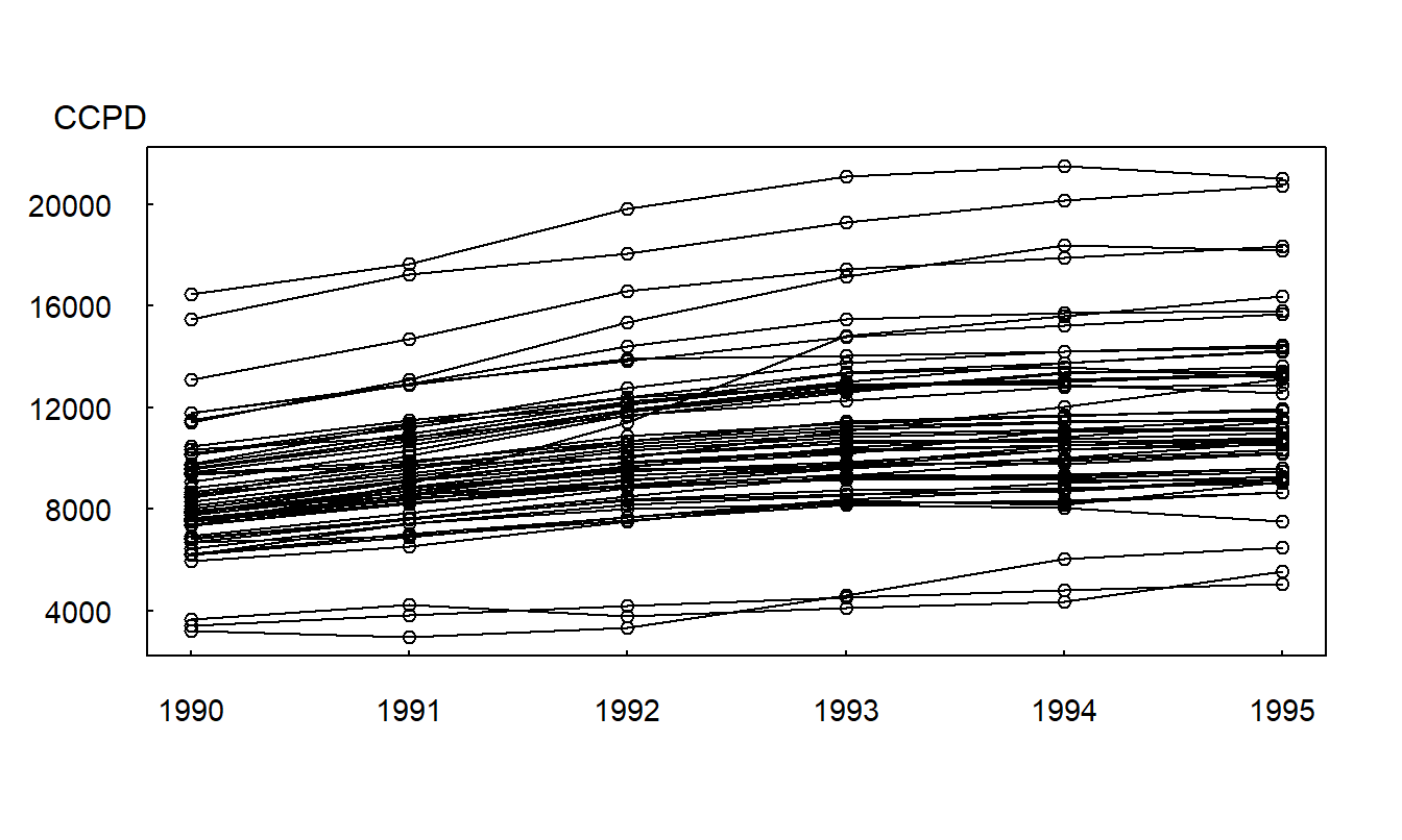
Figure 10.3: Multiple Time Series Plot of CCPD. Covered claims per discharge (CCPD) are plotted over \(T=6\) years, 1990-1995. The line segments connect states; thus, we see that CCPD increases for almost every state over time.
R Code to Produce Figure 10.3
Figure 10.4 is a variation of a scatter plot with symbols. This is a plot of CCPD versus number of discharges. One could use different plotting symbols each state; instead, we connect observations within a state over time. This plot shows a positive overall relationship between CCPD and the number of discharges. Like CCPD, we see a substantial state variation of different numbers of discharges. Also like CCPD, the number of discharges increases over time, so that, for each state, there is a positive relationship between CCPD and number of discharges. The slope is higher for those states with smaller number of discharges. This plot also suggests that the number of discharges lagged by one year is an important predictor of CCPD.
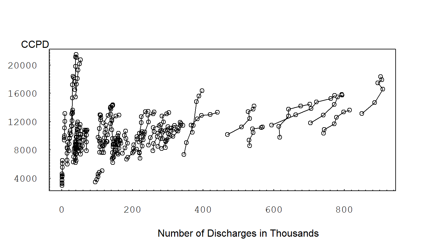
Figure 10.4: Scatter Plot of CCPD versus Number of Discharges. The line segments connect observations within a state over 1990-1995. We see a substantial state variation of numbers of discharges. There is a positive relationship between CCPD and number of discharges for each state. Slopes are higher for those states with smaller number of discharges.
R Code to Produce Figure 10.4
Trellis Plot
A technique for graphical display that has recently become popular in the statistical literature is a trellis plot. This graphical technique takes its name from a “trellis” which is a structure of open latticework. When viewing a house or garden, one typically thinks of a trellis as being used to support creeping plants such as vines. We will use this lattice structure and refer to a trellis plot as consisting of one or more panels arranged in a rectangular array. Graphs that contain multiple versions of a basic graphical form, each version portraying a variation of the basic theme, promote comparisons and assessments of change. By repeating a basic graphical form, we promote the process of communication.
Tufte (1997) states that using small multiples in graphical displays achieves the same desirable effects as using parallel structure in writing. Parallel structure in writing is successful because it allows readers to identify a sentence relationship only once and then focus on the meaning of each individual sentence element, such as a word, phrase or clause. Parallel structure helps achieve economy of expression and draw together related ideas for comparison and contrast. Similarly, small multiples in graphs allow us to visualize complex relationships across different groups and over time. See Guideline Five in Section 21.3 for further discussion.
Figure 10.5 illustrates the use of small multiples. In each panel, the plot portrayed is identical except that it is based on a different state; this use of parallel structure allows us to demonstrate the increasing covered claims per discharge (CCPD) for each state. Moreover, by organizing the states by average CCPD, we can see the overall level of CCPD for each state as well as variations in the slope (rate of increase).
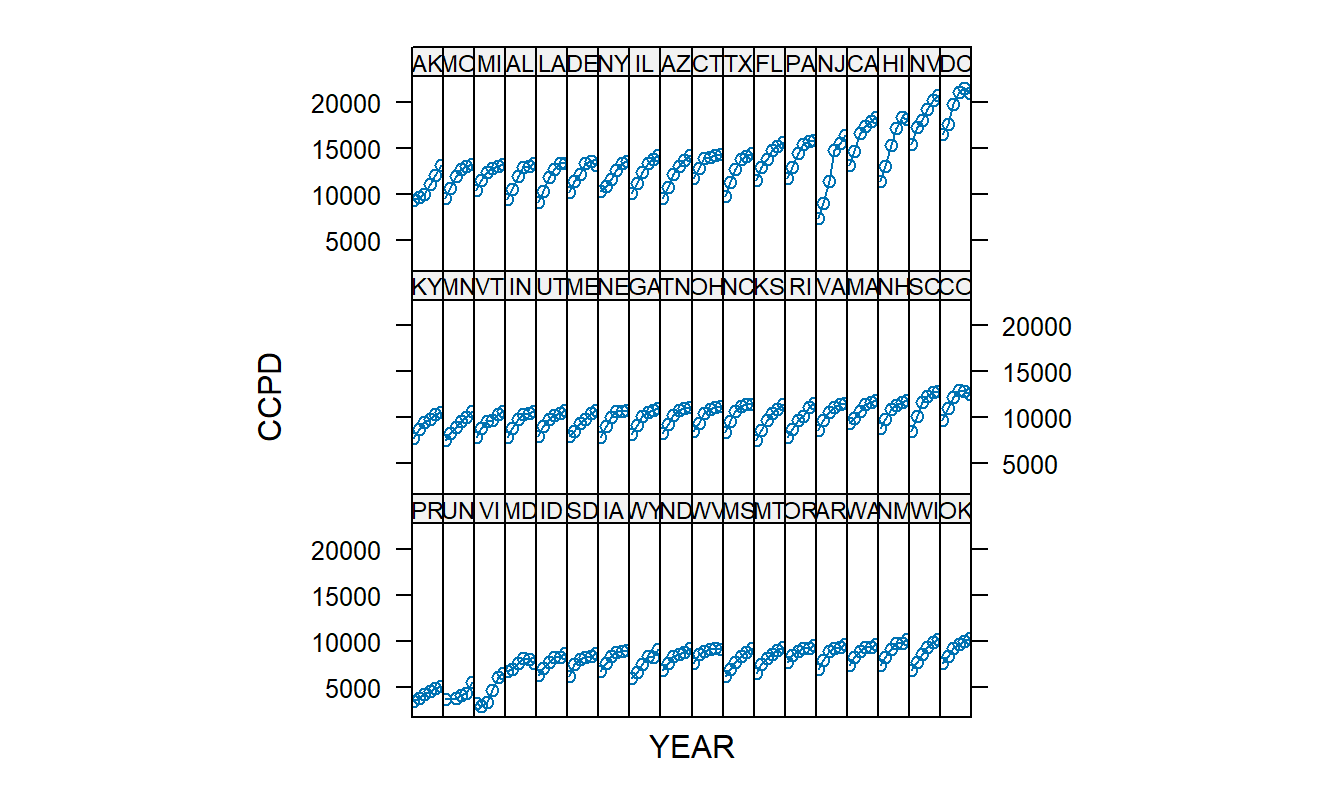
Figure 10.5: Trellis Plot of CCPD versus Year. Each of the 54 panels represents a plot of CCPD versus YEAR, 1990-1995 (the horizontal axis is suppressed). The increase for New Jersey (NJ) is unusually large.
R Code to Produce Figure 10.5
10.3 Basic Fixed Effects Models
Data
As described in Section 10.1, we let \(y_{it}\) denote the dependent variable of the \(i\)th subject at the \(t\)th time point. Associated with each dependent variable is a set of explanatory variables. For the state hospital costs example, these explanatory variables include the number of discharged patients and the average hospital stay per discharge. In general, we assume there are \(k\) explanatory variables \(x_{it,1}, x_{it,2}, \ldots, x_{it,k}\) that may vary by subject \(i\) and time \(t\). We achieve a more compact notational form by expressing the \(k\) explanatory variables as a \(k \times 1\) column vector \[ \mathbf{x}_{it} = \left(\begin{array}{c} x_{it,1} \\ x_{it,2} \\ \vdots \\ x_{it,k} \end{array}\right) . \]
With this notation, the data for the \(i\)th subject consists of: \[ \left(\begin{array}{c} x_{i1,1}, x_{i1,2}, \ldots, x_{i1,k}, y_{i1} \\ \vdots \\ x_{iT_i,1}, x_{iT_i,2}, \ldots, x_{iT_i,k}, y_{iT_i} \\ \end{array}\right) = \left(\begin{array}{c} \mathbf{x}_{i1}^{\prime}, y_{i1} \\ \vdots \\ \mathbf{x}_{iT_i}^{\prime}, y_{iT_i} \\ \end{array}\right) . \]
Model
A basic (and very useful) longitudinal data model is a special case of the multiple linear regression model introduced in Section 3.2. We use the modeling assumptions from Section 3.2.3 with the regression function \[\begin{eqnarray} \mathrm{E}~y_{it} & = & \alpha_i + \beta_1 x_{it,1} + \beta_2 x_{it,2} + \cdots + \beta_k x_{it,k} \nonumber\\ & = & \alpha_i + \mathbf{x}_{it}^{\prime} \boldsymbol \beta,~~~~~~ t=1, \ldots, T_i,~~ i=1, \ldots, n . \tag{10.1} \end{eqnarray}\] This is the basic fixed effects model.
The parameters \(\{\beta_j\}\) are common to each subject and are called global, or population, parameters. The parameters \(\{\alpha_i\}\) vary by subject and are known as individual, or subject-specific, parameters. In many applications, the population parameters capture broad relationships of interest and hence are the parameters of interest. The subject-specific parameters account for the different features of subjects, not broad population patterns. Hence, they are often of secondary interest and are called nuisance parameters. In Section 10.5, we will discuss the case where \(\{\alpha_i\}\) are random variables. To distinguish from this case, this section treats \(\{\alpha_i\}\) as non-stochastic parameters that are called “fixed effects.”
The subject-specific parameters help to control for differences, or “heterogeneity” among subjects. The estimators of these parameters use information in the repeated measurements on a subject. Conversely, the parameters \(\{\alpha_i\}\) are non-estimable in cross-sectional regression models without repeated observations. That is, with \(T_i\) = 1, the model \(y_{it} = \alpha_i + \beta_1 x_{it,1} + \beta_2 x_{it,2} + \cdots + \beta_k x_{it,k} + \varepsilon_{it}\) has more parameters (\(n+k\)) than observations (\(n\)) and thus, we cannot identify all the parameters. Typically, the disturbance term \(\varepsilon_{it}\) includes the information in \(\alpha_i\) in cross-sectional regression models. An important advantage of longitudinal data models when compared to cross-sectional regression models is the ability to separate the effects of \(\{\alpha_i\}\) from the disturbance terms \(\{\varepsilon_{it}\}\). By separating out subject-specific effects, our estimates of the variability become more precise and we achieve more accurate inferences.
Estimation
Estimation of the basic fixed effects model follows directly from the least squares methods. The key insight is that the heterogeneity parameters \(\{\alpha_i\}\) simply represent a factor, that is, a categorical variable that describes the unit of observation. With this, least squares estimation follows directly with the details given in Section 4.4 and the supporting appendices.
As described in Chapter 4, one can replace categorical variables with an appropriate set of binary variables. For this reason, panel data estimators are sometimes known as least squares dummy variable model estimators. However, as we have seen in Chapter 4, be careful on the statistical routines. For some applications, the number of subjects can easily run into the thousands. Creating this many binary variables is computationally cumbersome. When you identify a variable as categorical, statistical packages typically use more computationally efficient recursive procedures (described in Section 4.7.2).
The heterogeneity factor \(\{ \alpha_i \}\) does not depend on time. Because of this, it is easy to establish that regression coefficients associated with time-constant variables cannot be estimated using the basic fixed effects model. In other words, time-constant variables are perfectly collinear with the heterogeneity factor. Because of this limitation, analysts often prefer to design their studies to use the competing random effects model that we will describe in Section 10.5.
Example: Medicare Hospital Costs - Continued. We compare the fit of the basic fixed effects model to ordinary regression models. Model 1 of Table 10.1 shows the fit of an ordinary regression model using number of discharges (NUM_DCHG), YEAR and average hospital stay (AVE_DAYS). Judging by the large \(t\)-statistics, each variable is statistically significant. The intercept term is not printed.
Figure 10.5 suggests that New Jersey has an unusually large increase. Thus, an interaction term, YEARNJ, was created that equals YEAR if the observation is from New Jersey and zero otherwise. This variable is incorporated in Model 2 where it does not appear to be significant.
Table 10.1 also shows the fit of a basic fixed effects model with these explanatory variables. In the table, the 54 subject-specific coefficients are not reported. In this model, each variable is statistically significant, including the interaction term. Most striking is the improvement in the overall fit. The residual standard deviation (\(s\)) decrease from 2,731 to 530 and the coefficient of determination (\(R^2\)) increased from 29% to 99.8%.
Table 10.1. Coefficients and Summary Statistics from Three Models
\[ \small{ \begin{array} {lrrrrrr} \hline &\text{Regression}&&\text{Regression}&&\text{Basic Fixed} \\ &\text{Model 1} &&\text{Model 2} & &\text{Effects Model} \\ & \text{Coefficient} & t\text{-statistic} &\text{Coefficient} & t\text{-statistic} &\text{Coefficient} & t\text{-statistic} \\ \hline \text{NUM_DCHG} & 4.70 & 6.49 & 4.66 & 6.44 & 10.75 & 4.18 \\ \text{YEAR} & 744.15 & 7.96 & 733.27 & 7.79 & 710.88 & 26.51 \\ \text{AVE_DAYS} & 325.16 & 3.85 & 308.47 & 3.58 & 361.29 & 6.23 \\ \text{YEARNJ} & & & 299.93 & 1.01 & 1,262.46 & 9.82 \\ \hline s & {2,731.90} & & {2,731.78} & & {529.45} \\ R^2 \text{ (in percent)} & {28.6} & &{28.8} && {99.8} \\ R_a^2 \text{ (in percent)} & {27.9} && {27.9} && {99.8} \\ \hline \end{array} } \]
R Code to Produce Table 10.1
10.4 Extended Fixed Effects Models
Analysis of Covariance Models
In the basic fixed effects model, no special relationships between subjects and time periods are assumed. By interchanging the roles of “\(i\)” and “\(t\)”, we may consider the regression function \[ \mathrm{E}~y_{it} = \lambda_t + \mathbf{x}_{it}^{\prime} \boldsymbol \beta. \] Both this regression function and the one in equation (10.1) are based on traditional one-way analysis of covariance models introduced in Section 4.4. For this reason, the basic fixed effects model is also called the one-way fixed effects model. By using binary (dummy) variables for the time dimension, we can incorporate time-specific parameters into the population parameters. In this way, it is straightforward to consider the regression function \[ \mathrm{E}~y_{it} = \alpha_i + \lambda_t + \mathbf{x}_{it}^{\prime} \boldsymbol \beta , \] known as the two-way fixed effects model.
Example: Urban Wages. Glaeser and Maré (2001) investigated the effects of determinants on wages, with the goal of understanding why workers in cities earn more than their non-urban counterparts. They examined two-way fixed effects models using data from the National Longitudinal Survey of Youth (NLSY); they also used data from the Panel Study of Income Dynamics (PSID) to assess the robustness of their results to another sample. For the NLSY data, they examined \(n = 5,405\) male heads of households over the years 1983-1993, consisting of a total of \(N = 40,194\) observations. The dependent variable was logarithmic hourly wage. The primary explanatory variable of interest was a three level categorical variable that measures the city size in which workers reside. To capture this variable, two binary (dummy) variables were used: (1) a variable to indicate whether the worker resides in a large city (with more than one-half million residents), a “dense metropolitan area,” and (2) a variable to indicate whether the worker resides in a metropolitan area that does not contain a large city, a “non-dense metropolitan area.” The reference level is non-metropolitan area. Several other control variables were included to capture effects of a worker’s experience, occupation, education and race. When including time dummy variables, there were \(k = 30\) explanatory variables in the reported regressions.
Variable Coefficients Models
In the Medicare hospital costs example, we introduced an interaction variable to represent the unusually high increases in New Jersey costs. However, an examination of Figure 10.5 suggests that many other states are also “unusual.” Extending this line of thought, we might wish to allow each state to have its own rate of increase, corresponding to the increased hospital charges for that state. We could consider a regression function of the form \[\begin{equation} \small{ \mathrm{E}~CCPD_{it} = \alpha_i + \beta_1 (NUM\_DCHG)_{it} + \beta_{2i} (YEAR)_{t} + \beta_3 (AVE\_DAYS)_{it} , } \tag{10.2} \end{equation}\] where the slope associated with YEAR is allowed to vary with state “\(i\).”
Extending this line of thought, we write the regression function for a variable coefficients fixed effects model as \[ \mathrm{E}~y_{it} = \mathbf{x}_{it}^{\prime} \boldsymbol \beta_i. \] With this notation, we may allow any or all of the variables to be associated with subject-specific coefficients. For simplicity, the subject-specific intercept is now included in the regression coefficient vector \(\boldsymbol \beta_i\).
Example: Medicare Hospital Costs - Continued. The regression function in equation (10.2) was fit to the data. Not surprisingly, it resulted in excellent fit in the sense that the coefficient of determination is \(R^2 = 99.915 \%\) and the adjusted version is \(R_a^2 = 99.987 \%\). However, compared to the basic fixed effects model, there are an additional 52 parameters, a slope for each state (54 states to begin with, minus one for the `population’ term and minus one for New Jersey already included). Are the extra terms helpful? One way of analyzing this is through the general linear hypothesis test introduced in Section 4.2.2. In this context, the variable coefficients model represents the “full” equation and the basic fixed effects model is our “reduced” equation. From equation (4.4), the test statistic is \[ F-\textrm{ratio} = \frac {(0.99915 - 0.99809)/52}{(1-0.99915)/213} = 5.11 . \] Comparing this to the \(F\)-distribution with \(df_1 = 52\) and \(df_2 = 213\), we see that the associated \(p\)-value is less than 0.0001, indicating strong statistical significance. Thus, this is one indication that the variable slope model is preferred when compared to the basic fixed effects model.
Models with Serial Correlation
In longitudinal data, subjects are measured repeatedly over time. For some applications, time trends represent a minor portion of the overall variation. In these cases, one can adjust for their presence by calculating standard errors of regression coefficients robustly, similar to the Section 5.7.2 discussion. However, for other applications, getting a good understanding of time trends is vital. One such application that is important in actuarial science is prediction; for example, recall the Section 10.1 discussion of an actuary predicting insurance claims for a small business.
We have seen in Chapters 7–9 some basic ways to incorporate time trends, through linear trends in time (such as the YEAR term in the Medicare hospital costs example) or using dummy variables in time (another type of one-way fixed effects model). Another possibility is to use a lagged dependent variable as a predictor. However, this is known to have some unexpected negative consequences for the basic fixed effects model (see for example the discussion in Hsiao, 2003, Section 4.2 or Frees, 2004, Section 6.3).
Instead, it is customary to examine the serial correlation structure of the disturbance term \(\varepsilon_{it} = y_{it} - \mathrm{E}~y_{it}.\) For example, a common specification is to use an autocorrelation of order one, \(AR(1)\), structure, such as \[ \varepsilon_{it} = \rho_{\varepsilon} \varepsilon_{i,t-1} + \eta_{it}, \] where \(\{ \eta_{it} \}\) is a set of disturbance random variables and \(\rho_{\varepsilon}\) is the autocorrelation parameter. In many longitudinal datasets, the small number of time measurements (\(T\)) would inhibit calculation of the correlation coefficient \(\rho_{\varepsilon}\) using traditional methods such as those introduced in Chapter 8. However, with longitudinal data, we have many replications (\(n\)) of these short times series; intuitively, these replications provide the information needed to provide reliable estimates of the autoregressive parameter.
10.5 Random Effects Models
Suppose that you are interested in studying the behavior of subjects that are randomly selected from a population. For example, you might wish to predict insurance claims for a small business, using characteristics of the business as well as past claims history. Here, the set of small businesses may be randomly selected from a larger database. In contrast, the Section 10.3 Medicare example dealt with a fixed set of subjects. That is, it is difficult to think of the 54 states as a subset from some “super-population” of states. For both situations, it is natural to use subject-specific parameters, \(\{\alpha_i \}\), to represent the heterogeneity among subjects. Unlike Section 10.3, we now discuss situations in which it is more reasonable to represent \(\{\alpha_i \}\) as random variables instead of fixed, yet unknown, parameters. By arguing that \(\{\alpha_i \}\) are draws from a distribution, we will have the ability to make inferences about subjects in a population that are not included in the sample.
Basic Random Effects Model
The basic random effects model equation is \[\begin{equation} y_{it} = \alpha_i + \mathbf{x}_{it}^{\prime} \boldsymbol \beta + \varepsilon_{it},~~~~~~ t=1, \ldots, T_i,~~ i=1, \ldots, n . \tag{10.3} \end{equation}\] This notation is similar to the basic fixed effects model. However, now the term \(\alpha_i\) is assumed to be a random variable, not a fixed, unknown parameter. The term \(\alpha_i\) is known as a random effect. Mixed effects models are ones that include random as well as fixed effects. Because equation (10.3) includes random effects (\(\alpha_i\)) and fixed effects (\(\mathbf{x}_{it}\)), the basic random effects model is a special case of the mixed linear model. The general mixed linear model is introduced in Section 15.1.
To complete the specification, we assume that \(\{\alpha_i \}\) are identically and independently distributed with mean zero and variance \(\sigma_{\alpha}^2\). Further, we assume that \(\{\alpha_i \}\) are independent of the disturbance random variables, \(\varepsilon_{it}\). Note that because E \(\alpha_i\) = 0, it is customary to include a constant within the vector \(\mathbf{x}_{it}\). This was not true of the fixed effects models in Section 10.3 where we did not center the subject-specific terms about 0.
Linear combinations of the form \(\mathbf{x}_{it}^{\prime} \boldsymbol \beta\) quantify the effect of known variables that may affect the dependent variable. Additional variables, that are either unimportant or unobservable, comprise the “error term.” In equation (10.3), we may think of a regression model \(y_{it} = \mathbf{x}_{it}^{\prime} \boldsymbol \beta + \eta_{it},\) where the error term \(\eta_{it}\) is decomposed into two components so that \(\eta_{it}= \alpha_i + \varepsilon_{it}\). The term \(\alpha_i\) represents the time-constant portion whereas \(\varepsilon_{it}\) represents the remaining portion. To identify the model parameters, we assume that the two terms are independent. In the econometrics literature, this is known as the error components model; in the biological sciences, is is known as the random intercepts model.
Estimation
Estimation of the random effects model does not follows directly from least squares as with the fixed effects models. This is because the observations are no longer independent due to the random effects terms. Instead, an extension of least squares known as generalized least squares is used to account for this dependency. Generalized least squares, often denoted by the acronym GLS, is a type of weighted least squares. Because random effects models are special cases of mixed linear models, we will introduce GLS estimation in this broader framework in Section 15.1.
To see the dependency among observations, consider the covariance between the first two observations of the \(i\)th subject. Basic calculations show
\[\begin{eqnarray*} \mathrm{Cov}(y_{i1}, y_{i2}) &= &\mathrm{Cov}(\alpha_i + \mathbf{x}_{i1}^{\prime} \boldsymbol \beta + \varepsilon_{i1}, \alpha_i + \mathbf{x}_{i2}^{\prime} \boldsymbol \beta + \varepsilon_{i2}) \\ &= &\mathrm{Cov}(\alpha_i +\varepsilon_{i1}, \alpha_i + \varepsilon_{i2}) \\&= &\mathrm{Cov}(\alpha_i , \alpha_i)+\mathrm{Cov}(\alpha_i, \varepsilon_{i2})+\mathrm{Cov}(\varepsilon_{i1}, \alpha_i)+\mathrm{Cov}(\varepsilon_{i1}, \varepsilon_{i2}) \\ &= & \mathrm{Cov}(\alpha_i , \alpha_i) = \sigma^2_{\alpha} . \end{eqnarray*}\] The systematic terms \(\mathbf{x}^{\prime} \boldsymbol \beta\) drop out of the covariance calculation because they are non-random. Further, the covariance terms involving \(\varepsilon\) are zero because of the assumed independence. This calculation shows that the covariance between any two observations from the same subject is \(\sigma^2_{\alpha}\). Similar calculations show that the variance of an observation is \(\sigma^2_{\alpha} +\sigma^2_{\varepsilon}.\) Thus, the correlation between observations within a subject is \(\sigma^2_{\alpha} / (\sigma^2_{\alpha} +\sigma^2_{\varepsilon})\). This quantity is known as the intra-class correlation, a commonly reported measure of dependence in random effects studies.
Example: Group Term Life. Frees, Young and Luo (2001) analyzed claims data provided by an insurer of credit unions. The data contains claims and exposure information from 88 Florida credit unions for years 1993-1996. These are “life savings” claims from a contract between the credit union and their members that provides a death benefit based on the member’s savings deposited in the credit union. Actuaries typically price life insurance coverage with knowledge of an insureds’ age and gender, as well as other explanatory variables such as occupation. However, for these data from small groups, often only a minimal amount of information is available to understand claims behavior.
Of the \(88 \times 4=352\) potential observations, 27 were not available because these credit unions had zero coverage in that year (and thus excluded). Thus, these data were unbalanced. The dependent variable is the annual total claims from the life savings contract, in logarithmic units. The explanatory variables were annual coverage, in logarithmic units, and YEAR, a time trend.
A fit of the basic random effects model showed that both year and the annual coverage had positive and strongly statistically significant coefficients. That is, the typical amount of claims increased over the period studied and claims increased as coverage increased, other things being equal. There were strong credit union effects, as well. For example, the estimated intra-class correlation was 0.703, also suggesting strong dependence among observations.
Extended Random Effects Models
Just as with fixed effects, random effects models can be easily extended to incorporated variable coefficients and serial correlations. For example, Frees et al. (2001) considered the model equation \[\begin{equation} y_{it} = \alpha_{1i} + \alpha_{2i} \mathrm{LNCoverage}_{it}+ \beta_1 + \beta_2 \mathrm{YEAR}_t+ \beta_3 \mathrm{LNCoverage}_{it}+ \varepsilon_{it} , \tag{10.4} \end{equation}\] where \(\mathrm{LNCoverage}_{it}\) is the logarithmic life savings coverage. As with the basic model, it is customary to use a mean zero for the random effects. Thus, the overall intercept is \(\beta_1\) and \(\alpha_{1i}\) represents credit union deviations. Further, the overall or global slope associated with \(\mathrm{LNCoverage}\) is \(\beta_3\) and \(\alpha_{2i}\) represents credit union deviations. Put another way, the slope corresponding to \(\mathrm{LNCoverage}\) for the \(i\)th credit is \(\beta_3 + \alpha_{2i}\).
More generally, the variable coefficients random effects model equation can be written as \[\begin{equation} y_{it} = \mathbf{x}_{it}^{\prime} \boldsymbol \beta + \mathbf{z}_{it}^{\prime} \boldsymbol \alpha _i + \varepsilon_{it}. \tag{10.5} \end{equation}\] As with the fixed effects variable coefficients model, we may allow any or all of the variables to be associated with subject-specific coefficients. The convention used in the literature is to specific fixed effects through the systematic component \(\mathbf{x}_{it}^{\prime} \boldsymbol \beta\) and random effects through the component \(\mathbf{z}_{it}^{\prime} \boldsymbol \alpha _i\). Here, the vector \(\mathbf{z}_{it}\) is typically equal to or a subset of \(\mathbf{x}_{it}\) although it need not be so. With this notation, we now have a vector of random effects \(\boldsymbol \alpha _i\) that are subject-specific. To reduce to our basic model, one only needs to choose \(\boldsymbol \alpha _i\) to be a scalar (a \(1 \times 1\) vector) and \(\mathbf{z}_{it}\equiv 1.\) The example in equation (10.4) results from choosing \(\boldsymbol \alpha _i = (\alpha_{1i}, \alpha_{2i})^{\prime}\) and \(\mathbf{z}_{it} = (1, \mathrm{LNCoverage}_{it})^{\prime}\).
As with fixed effects models, one can readily incorporate models of serial correlation into random effects models by specifying a correlations structure for \(\varepsilon_{i1}, \ldots, \varepsilon_{iT}\). This feature is readily available in statistical packages and is described fully in the Section 10.6 references.
10.6 Further Reading and References
Longitudinal and panel data models are widely used. To illustrate, an index of business and economic journals, ABI/INFORM, lists 685 articles in 2004 and 2005 that use panel data methods. Another index of scientific journals, the ISI Web of Science, lists 1,137 articles in 2004 and 2005 that use longitudinal data methods. A book-long introduction to longitudinal and panel data that emphasizes business and social science applications is Frees (2004). Diggle et al. (2002) provides an introduction from a biomedical perspective. Hsiao (2003) provides a classic introduction from an econometric perspective.
Actuaries are particularly interested in predictions resulting from longitudinal data. These predictions can form the basis for updating insurance prices. This topic is discussed in Chapter 18 on credibility and bonus-malus factors.
Chapter References
- Diggle, Peter J., Patrick Heagarty, Kung-Yee Liang and Scott L. Zeger (2002). Analysis of Longitudinal Data, Second Edition. Oxford University Press, London.
- Frees, Edward W. (2004). Longitudinal and Panel Data: Analysis and Applications in the Social Sciences. Cambridge University Press, New York.
- Frees, Edward W., Virginia R. Young and Yu Luo (2001). Case studies using panel data models. North American Actuarial Journal 5 (4), 24-42.
- Glaeser, E. L. and D. C. Maré (2001). Cities and skills. Journal of Labor Economics 19, 316-342.
- Hsiao, Cheng (2003). * Analysis of Panel Data, Second Edition*. Cambridge University Press, New York.
- Tufte, Edward R. (1997). Visual Explanations. Cheshire, Conn.: Graphics Press.