Chapter 18 Credibility and Bonus-Malus
Chapter Preview. This chapter introduces regression applications of pricing in credibility and bonus-malus experience rating systems. Experience rating systems are formal methods for including claims experience into renewal premiums of short-term contracts, such automobile, health and workers compensation. This chapter provides brief introductions to credibility and bonus-malus, emphasizing their relationship with regression methods.
18.1 Risk Classification and Experience Rating
Risk classification is a key ingredient of insurance pricing. Insurers sell coverage at prices that are sufficient to cover anticipated claims, administrative expenses and an expected profit to compensate for the cost of capital necessary to support the sale of the coverage. In many countries and lines of business, the insurance market is mature and highly competitive. This strong competition induces insurers to classify risks they underwrite in order to receive fair premiums for the risk undertaken. This classification is based on known characteristics of the insured, the person or firm seeking the insurance coverage.
For example, suppose that you are working for a company that insures small businesses for time lost due to employees injured on the job. Consider pricing this insurance product for two businesses that are identical with respect to number of employees, location, age and gender distribution and so forth, except that one company is a management consulting firm and the other is a construction firm. Based on experience, you expect the management consulting firm to have a lower claims level than the construction firm and you need to price accordingly. If you do not, another insurance company will offer a lower insurance price to the consulting firm and take this potential customer away, leaving your company with only the more costly construction firm business.
Competition among insurers leads to charging premiums according to observable characteristics, known as risk classification. In the context of regression modeling, we can think of this as modeling the claims distributions in terms of explanatory variables.
Many pricing situations are based on a relationship between the insurer and the insured that develops over time. These relationships allow insurers to base prices on unobservable characteristics of the insured by taking into account the prior claims experience of the insured. Modifying premiums with claims history is known as experience rating, also sometimes referred to as merit rating.
Experience rating methods are either applied retrospectively or prospectively. With retrospective methods, a “refund” of a portion of the premium is provided to the insured in the event of favorable (to the insurer) experience. Retrospective premiums are common in life insurance arrangements (where insureds earned “dividends” in the U.S. and “bonuses” in the U.K.). In property and casualty insurance prospective methods are more common, where favorable insured experience is “rewarded” through a lower renewal premium.
In this chapter, we discuss two prospective methods that are well-suited for regression modeling, credibility and bonus-malus. Bonus-malus methods are used extensively in Asia and Europe, although almost exclusively with automobile insurance. As we will see in Section 18.4, the idea is to use claims experience to modify the classification of an insured. Credibility methods, introduced in Section 18.2, are more broadly applied in terms of lines of business and geography.
18.2 Credibility
Credibility is a technique for pricing insurance coverages that is widely used by health, group term life and property and casualty actuaries. In the United States, the standards are described under the Actuarial Standard of Practice Number 25 published by the Actuarial Standards Board of the American Academy of Actuaries (web site: http://www.actuary.org/). Further, several insurance laws and regulation require the use of credibility.
The theory of credibility has been called a “cornerstone” of the field of actuarial science (Hickman and Heacox, 1999). The basic idea is to use claims experience and additional information to develop a pricing formula, such as through the relation \[\begin{equation} New~Premium = \zeta \times Claims~Experience + (1 - \zeta) \times Old~Premium. \tag{18.1} \end{equation}\] Here, \(\zeta\) (the Greek letter “zeta”) is known as the “credibility factor;” values generally lie between zero and one. The case \(\zeta=1\) is known as “full credibility,” where claims experience is used solely to determine the premium. The case \(\zeta=0\) can be thought of as “no credibility,” where claims experience is ignored and external information is used as the sole basis for pricing.
To keep this chapter self-contained, we begin by introducing some basic credibility concepts. Section 18.2.1 reviews classic concepts of credibility, including when to use it and linear pricing formulas. Section 18.2.2 describes the modern version of credibility by introducing a formal probabilistic model that can be used for updating insurance prices. Section 18.3 discusses the link with regression modeling.
18.2.1 Limited Fluctuation Credibility
Credibility has a long history in actuarial science, with fundamental contributions dating back to Mowbray (1914). Subsequently, Whitney (1918) introduced the intuitively appealing concept of using a weighted average of (1) claims from the risk class and (2) claims over all risk classes to predict future expected claims.
Standards for Full Credibility
The title of Mowbray’s paper was “How extensive a payroll exposure is necessary to give a dependable pure premium?” It is still the first question that an analyst needs to confront: when do I need to use credibility estimators? To get a better handle on this question, consider the following situation.
Example: Dental Costs. Suppose that you are pricing dental insurance coverage for a small employer. For males aged 18-25, the employer provides the following experience:
\[ \small{ \begin{array}{l|rrr} \hline \text{Year} & 2007 & 2008 & 2009 \\ \hline \text{Number} & 8 & 12 & 10 \\ \text{Average Dental Cost} & 500 & 400 & 900 \\ \hline \end{array} } \]
The “manual rate,” available from a tabulation of a much larger set of data, is $700 per employee. Ignoring inflation and expenses, what would you use to anticipate dental costs in 2010? The manual rate? The average of the available data? Or some combination?
Mowbray wanted to distinguish between situations when (1) large employers with substantial information could use their own experience and (2) small employers with limited experience would use external sources, so-called “manual rates.” In statistical terminology, we can think about forming an estimator from an employer’s experience of the true mean costs. We are asking whether the distribution of the estimator is sufficiently close to the mean to be reliable. Of course, “sufficiently close” is the tricky part, so let us look at a more concrete situation.
The simplest set-up is to assume that you have claims \(y_1, \ldots, y_n\) that are identically and independently distributed (i.i.d.) with mean \(\mu\) and variance \(\sigma^2\). As a standard for full credibility, we could require that \(n\) be large enough so that
\[\begin{equation} \Pr ( (1-r) \mu \leq \bar{y} \leq (1+r) \mu) \geq p, \tag{18.2} \end{equation}\] where \(r\) and \(p\) are given constants. For example, if \(r=0.05\) and \(p=0.9\), then we wish to have at least 90% chance of being within 5% of the mean.
Using normal approximations, it is straight-forward to show that sufficient for equation (18.2) is
\[\begin{equation} n \geq \left(\frac{\Phi^{-1}(\frac{p+1}{2}) \sigma}{r \mu} \right)^2 . \tag{18.3} \end{equation}\] We define \(n_F\), the number of observations required for full credibility, to be the smallest value of \(n\) that satisfies equation (18.3).
Example: Dental Costs - Continued. From the table, average costs are \(\bar{y} = \left( 500 \times 8 + 400 \times 12 + 900 \times 10 \right)/30 = 593.33.\) Suppose that we have available an estimate of the standard deviation \(\sigma \approx \widehat{\sigma}= 200.\) Using \(p=0.90\), the 90th percentile of the normal distribution is \(\Phi^{-1}(.95) = 1.645\). With \(r=0.05\), the approximate sample size required is \[ \left(\frac{\Phi^{-1}(.95) \widehat{\sigma}}{r \bar{y}} \right)^2 = \left(\frac{1.645 \times 200}{0.05 \times 593.33} \right)^2= 122.99, \] or \(n_F=123\). Based on a sample of size 30, we do not have enough observations for full credibility.
The standards for full credibility given in equations (18.2) and (18.3) are based on approximate normality. It is easy to construct similar rules for other distributions such as binomial and Poisson count data or mixtures of distributions for aggregate losses. See Klugman, Panjer and Willmot (2008) for more details.
Partial Credibility
Actuaries do not always work with massive data sets. You may be working with the experience from a small employer or association and not have sufficient experience to meet the full credibility standard. Or, you may be working with a large employer but have decided to decompose your data into small, homogeneous subsets. For example, if you are working with dental claims, you may wish to create several small groups based on age and gender.
For smaller groups that do not meet the full credibility threshold, Witney (1918) proposed using a weighted average of the group’s claims experience and a manual rate. Assuming approximate normality, the expression for partial credibility is \[\begin{equation} New~Premium = Z \times \bar{y} + (1 - Z) \times Manual~Premium, \tag{18.4} \end{equation}\] where \(Z\) is the “credibility factor,” defined as \[\begin{equation} Z = \min{\LARGE\{}1,\sqrt{\frac{n}{n_F}} ~~{\LARGE\}}. \tag{18.5} \end{equation}\] Here, \(n\) is the sample size and \(n_F\) is the number of observations required for full credibility.
Example: Dental Costs - Continued. From prior work, the standard for full credibility is \(n_F = 123\). Thus, the credibility factor is \(\min\{1,\sqrt{\frac{30}{123}} \} = 0.494.\) With this, the partial credibility premium is \[ New~Premium = 0.494 \times 593.33 + (1 - 0.494) \times 700 = 647.31. \]
One line of justification for the partial credibility formulas in equations (18.4) and (18.5) is given in the exercises. From equation (18.5), we see that the credibility factor \(Z\) is bounded by 0 and 1; as the sample size \(n\) and hence the experience becomes larger, \(Z\) tends to 1. This means that larger groups are more “credible.” As the credibility factor \(Z\) increases, a greater weight is placed upon the group’s experience (\(\bar{y}\)). As \(Z\) decreases, more weight is placed upon the manual premium, the rate that is developed externally based on the group’s characteristics.
18.2.2 Greatest Accuracy Credibility
Credibility theory was used for over fifty years in insurance pricing before it was placed on a firm mathematical foundation by Bühlmann (1967). To introduce this framework, sometimes known as “greatest accuracy credibility,” let us begin with the assumption that we have a sample of claims \(y_1, \ldots, y_n\) from a small group and that we wish to estimate the mean for this group. Although the sample average \(\bar{y}\) is certainly a sensible estimator, the sample size may be too small to rely exclusively on \(\bar{y}\). We also suppose that have an external estimate of overall mean claims, \(M\), that we think of as a “manual premium.” The question is whether we can combine the two estimates, \(\bar{y}\) and \(M\), to provide an estimator that is superior to either alternative.
Bühlmann hypothesized the existence of unobserved characteristics of the group that we denote as \(\alpha\); he referred to these as “structure variables.” Although unobserved, these characteristics are common to all observations from the group. For dental claims, the structure variables may include the water quality where the group is located, the number of dentists to provide preventative care in the area, the educational level of the group, and so forth. Thus, we assume, conditional on \(\alpha\), that \(\{y_1, \ldots, y_n\}\) are a random sample from an unknown population and hence are i.i.d. For notation, we will let \(\mathrm{E}(y | \alpha)\) denote the conditional expected claims and \(\mathrm{Var}(y | \alpha)\) to be the corresponding conditional variance. Our goal is to determine a sensible “estimator” of \(\mathrm{E}(y | \alpha)\).
Although unobserved, we can learn something about the characteristics \(\alpha\) from repeated observations of claims. For each group, the (conditional) mean and variance functions are \(\mathrm{E}(y | \alpha)\) and \(\mathrm{Var}(y | \alpha)\), respectively. The expectation over all groups of the variance functions is E \(\mathrm{Var}(y | \alpha)\). Similarly, the variance of conditional expectations is Var \(\mathrm{E}(y | \alpha)\).
With these quantities in hand, we are able to give Bühlmann’s credibility premium. \[\begin{equation} New~Premium = \zeta \times \bar{y} + (1 - \zeta) \times M, \tag{18.6} \end{equation}\] where \(\zeta\) is the “credibility factor,” defined as \[\begin{equation} \zeta = \frac{n}{n+Ratio}, ~\mathrm{with}~~~~~~~~Ratio = \frac{\mathrm{E~}\mathrm{Var}(y | \alpha)}{\mathrm{Var}~\mathrm{E}(y | \alpha)}. \tag{18.7} \end{equation}\] The credibility formula in equation (18.6) is the same as the classic partial credibility formula in equation (18.4), with the credibility factor \(\zeta\) in place of \(Z\). Thus, it shares the same intuitively pleasing expression as a weighted average. Further, both credibility factors lie in the interval \((0,1)\) and both increase to one as the sample size \(n\) increases.
Example: Dental Costs - Continued. From prior work, we have that an estimate of the conditional mean is 593.33. Use similar calculations to show that the estimated conditional variance is 48,622.22.
Now assume that there are three additional groups with conditional means and variances given as follows:
\[ \small{ \begin{array}{c|cccc} \hline & & \text{Conditional} & \text{Conditional } \\ & \text{Unobserved} & \text{Mean } & \text{Variance} & \text{Probability} \\ \text{Group}& \text{Variable} & \text{E} (y|\alpha)& \text{Var} (y|\alpha) & \Pr(\alpha) \\ \hline 1 & \alpha_1 & 593.33 & 48,622.22 & 0.20 \\ 2 & \alpha_2& 625.00 & 50,000.00 & 0.30 \\ 3 & \alpha_3& 800.00 & 70,000.00 & 0.25 \\ 4 & \alpha_4& 400.00 & 40,000.00 & 0.25 \\ \hline \end{array} } \] We assume that probability of being a member of a group is given as \(\Pr(\alpha)\). For example, this may be determined by taking proportions of the number of members in each group.
With this information, it is straight-forward to calculate the expected conditional variance, \[ \mathrm{E~}\mathrm{Var}(y | \alpha) = 0.2(48622.22) + 0.3(50000) + .25(70000) + .25(40000) = 52,224.44 . \]
To calculate the variance of conditional expectations, one can begin with the overall expectation \[ \mathrm{E~}\mathrm{E}(y | \alpha) = 0.2(593.33) + 0.3(625) + .25(800) + .25(400) = 606.166, \] and then use a similar procedure to calculate the expected value of the conditional second moment, \(\mathrm{E~}(\mathrm{E}(y | \alpha))^2 = 387,595.6\). With these two pieces, the variance of conditional expectations is \(\mathrm{E~}\mathrm{Var}(y | \alpha)\) \(= 387,595.6- 606.166^2 = 20,158.\)
This yields the \(Ratio=52224.44/20158 = 2.591\) and thus the credibility factor \(\zeta = \frac{30}{30+2.591} = 0.9205\). With this, the credibility premium is \[ New~Premium = 0.9205 \times 593.33 + (1 - 0.9205) \times 700 = 601.81. \]
To see how to use the credibility formula using alternative distributions, consider the following.
Example: Credibility with Count Data. Suppose that the number of claims each year for an individual insured has a Poisson distribution. The expected annual claim frequency of the entire population of insureds is uniformly distributed over the interval (0,1). An individual’s expected claims frequency is constant through time.
Consider a particular insured that had 3 claims during the prior three years.
Under these assumptions, we have the claims for an individual \(y\) with latent characteristics \(\alpha\) are Poisson distributed with conditional mean \(\alpha\) and conditional variance \(\alpha\). The distribution of \(\alpha\) is uniform on the interval (0,1), so easy calculations show that \[ \mathrm{E}~\mathrm{Var}(y|\alpha) = \mathrm{E}~\alpha = 0.5~~~\mathrm{and}~~~ \mathrm{Var}~\mathrm{E}(y|\alpha) = \mathrm{Var}~\alpha = 1/12 = 0.08333. \] Thus, with \(n=3\), the credibility factor is \[ \zeta = \frac{3}{3+ 0.5/0.08333} = 0.3333. \] With \(\bar{y}=3/3 =1\) and the overall mean \(\mathrm{E}~\mathrm{E}(y|\alpha)=0.5\) as the manual premium, the credibility premium is \[ New~Premium = 0.3333 \times 1 + (1 - 0.3333) \times 0.5 = 0.6667. \]
More formally, the optimality of the credibility estimator is based on the following.
Property. Assume, conditional on \(\alpha\), that \(\{y_1, \ldots, y_n \}\) are identically and independently distributed with conditional mean and variance \(\mathrm{E}(y | \alpha)\) and and \(\mathrm{Var}(y | \alpha)\), respectively. Suppose that we wish to estimate \(\mathrm{E}~(y_{n+1}|\alpha)\). Then, the credibility premium given in equations (18.6) and (18.7) has the smallest variance within the class of all linear unbiased predictors.
This property indicates that the credibility premium has “greatest accuracy” in the sense that it has minimum variance among linear unbiased predictors. As we have seen, it is couched in terms of means and variances that can be applied to many distributions; unlike the partial credibility premium, there is no assumption of normality. It is a fundamental result in that it is based on (conditionally) i.i.d. observations. Not surprisingly, it is easy to modify this basic result to allow for different exposures for observations, trends in times and so forth.
The property is silent on how one would estimate quantities associated with the distribution of \(\alpha\). To do this, we will introduce a more detailed sampling scheme that will allow us to incorporate regression methods. Although not the only way of sampling, this framework will allow us to introduce many variations of interest and will help to interpret credibility in a natural way.
18.3 Credibility and Regression
By expressing credibility in the framework of regression models, actuaries can realize several benefits:
- Regression models provide a wide variety of models from which to choose.
- Standard statistical software makes analyzing data relatively easy.
- Actuaries have another method for explaining the ratemaking process.
- Actuaries can use graphical and diagnostic tools to select a model and assess its usefulness.
18.3.1 One-Way Random Effects Model
Assume that we are interested in pricing for \(n\) groups and that for each of the \(i=1,\ldots,n\) groups, we have claims experience \(y_{it}, t=1, \ldots, T\). Although this is the longitudinal data set-up introduced in Chapter 10, we need not assume that claims evolve over time; the \(t\) subscripts may represent different members of a group. To begin, we assume that we do not have an explanatory variables. Claims experience follows \[\begin{equation} y_{it} = \mu + \alpha_i + \varepsilon_{it}, ~~~~~ t=1, \ldots, T, i=1,\ldots, n, \tag{18.8} \end{equation}\] where \(\mu\) represents an overall claim average, \(\alpha_i\) the unobserved group characteristics and \(\varepsilon_{it}\) the individual claim variation. We assume that \(\{\alpha_i\}\) are i.i.d. with mean zero and variance \(\sigma^2_{\alpha}\). Further assume that \(\{\varepsilon_{it}\}\) are i.i.d. with mean zero and variance \(\sigma^2\) and are independent of \(\alpha_i\). These are the assumptions of a basic “one-way random effects” model described in Section 10.5.
It seems reasonable to use the quantity \(\mu + \alpha_i\) to predict a new claim from the \(i\)th group. For the model in equation (18.8), it seems intuitively plausible that \(\bar{y}\) is a desirable estimator of \(\mu\) and that \(\bar{y}_i-\bar{y}\), is a desirable “estimator” of \(\alpha_i\). Thus, \(\bar{y}_i\) is a desirable predictor of \(\mu+\alpha_i\). More generally, consider predictors of \(\mu+\alpha_i\) that are linear combinations of \(\bar{y}_i\) and \(\bar{y}\), that is, \(c_1 \bar{y}_i+c_2\bar{y}\), for constants \(c_1\) and \(c_2\). To retain the unbiasedness, we use \(c_2 = 1 - c_1\). Some basic calculations show that the best value of \(c_1\) that minimizes \(\mathrm{E} \left( c_1 \bar{y}_i+(1-c_1)\bar{y} - (\mu+\alpha_i) \right)^2\) is \[ c_1 = \frac{T}{T+\sigma^2/\sigma^2_{\alpha}} = \zeta, \] the credibility factor. This yields the shrinkage estimator, or predictor, of \(\mu+\alpha_i\), defined as \[\begin{equation} \bar{y}_{i,s} = \zeta \bar{y}_i+(1-\zeta)\bar{y}. \tag{18.9} \end{equation}\]
The shrinkage estimator is equivalent to credibility premium when we see that \[ \mathrm{Var} \left(\mathrm{E}(y_{it}|\alpha_i) \right) = \mathrm{Var} \left(\mathrm{E}(\mu+\alpha_i) \right) = \sigma^2_{\alpha} \] and \[ \mathrm{E} \left(\mathrm{Var}(y_{it}|\alpha_i) \right) = \mathrm{E} \left(\mathrm{E}(\sigma^2) \right) = \sigma^2 , \] so that \(Ratio = \sigma^2/\sigma^2_{\alpha}\). Thus, the one-way random effects model is sometimes referred to as the “balanced Bühlmann” model. This shrinkage estimator is also a best linear unbiased predictor (\(BLUP\)), introduced in Section 15.1.3.
Example: Visualizing Shrinkage. Consider the following illustrative data:
\[ \small{ \begin{array}{c|cccc|c} \hline \text{Group}&&&&&\text{Group}\\ i& 1 & 2 & 3 & 4 & \text{Average } (\bar{y}_i)\\ \hline 1 & 14 & 12 & 10 & 12 & 12 \\ 2 & 9 & 16 & 15 & 12 & 13 \\ 3 & 8 & 10 & 7 & 7 & 8 \\ \hline \end{array} } \]
That is, we have \(n=3\) groups, each of which has \(T=4\) observations. The sample mean is \(\bar{y} = 11\) and group-specific sample means are \(\bar{y}_1=12\), \(\bar{y}_2=13\) and \(\bar{y}_3=8\). We now fit the one-way random effects ANOVA model in equation (18.8) using maximum likelihood estimation assuming normality. Standard statistical software shows that the estimates of \(\sigma^2\) and \(\sigma^2_{\alpha}\) are 4.889 and 5.778, respectively. It follows that the estimated \(\zeta\) factor is 0.738. Using equation (18.9), the corresponding predictions for the subjects are 11.738, 12.476, and 8.786, respectively.
Figure 18.1 compares group-specific means to the corresponding predictions. Here, we see less spread in the predictions compared to the group-specific means; each group’s estimate is “shrunk” to the overall mean, \(\bar{y}\) . These are the best predictors assuming \(\alpha_i\) are random. In contrast, the subject-specific means are the best predictors assuming \(\alpha_i\) are deterministic. Thus, this “shrinkage effect” is a consequence of the random effects specification.
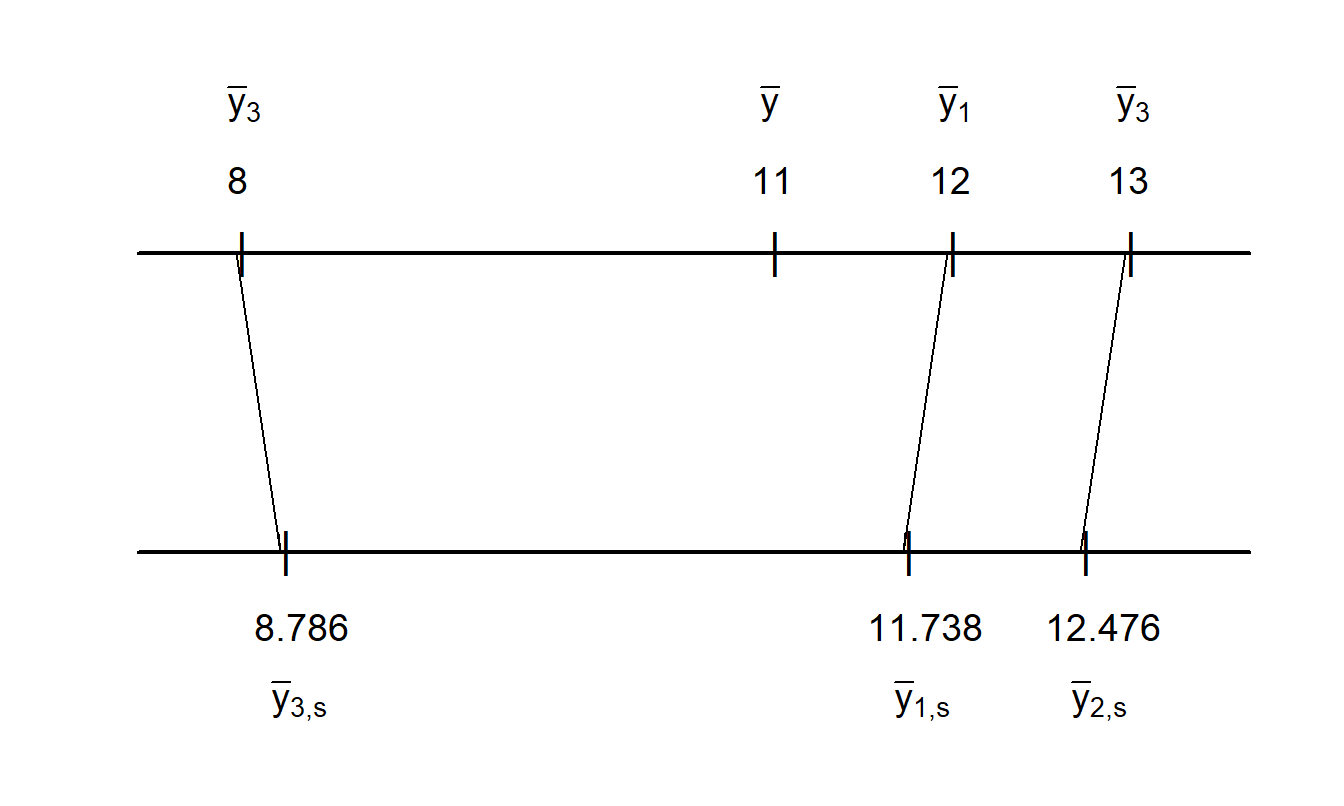
Figure 18.1: Comparison of Group-Specific Means to Shrinkage Estimates. For an illustrative data set, group-specific and overall means are graphed on the upper scale. The corresponding shrinkage estimates are graphed on the lower scale. This figure shows the shrinkage aspect of models with random effects.
Under the one-way random effects model, we have that \(\bar{y}_i\) is an unbiased predictor of \(\mu+\alpha_i\) in the sense that E (\(\bar{y}_i - (\mu+\alpha_i)\))=0. However, \(\bar{y}_i\) is inefficient in the sense that the shrinkage estimator, \(\bar{y}_{i,s}\), has a smaller mean square error than \(\bar{y}_i\). Intuitively, because \(\bar{y}_{i,s}\) is a linear combination of \(\bar{y}_i\) and \(\bar{y}\), we say that has been “shrunk” towards the estimator \(\bar{y}\). Further, because of the additional information in \(\bar{y}_{i,s}\), it is customary to interpret a shrinkage estimator as “borrowing strength” from the estimator of the overall mean.
Note that the shrinkage estimator reduces to the fixed effects estimator \(\bar{y}_i\) when the credibility factor, \(\zeta\), becomes 1. It is easy to see that \(\zeta \rightarrow 1\) as either (i) \(T\rightarrow\infty\) or (ii) \(\sigma^2/\sigma^2_{\alpha}\rightarrow 0\). That is, the best predictor approaches the group mean as either (i) the number of observations per group becomes large or (ii) the variability among groups becomes large relative to the response variability. In actuarial language, either case supports the idea that the information from the \(i\)th group is becoming more “credible.”
18.3.2 Longitudinal Models
As we have seen the context of the one-way random effects model with balanced replications, Bühlmann’s greatest accuracy credibility estimator is equivalent to the best linear unbiased predictor introduced in Section 15.1.3. This is also true when considering a more general longitudinal sampling set-up introduced in Chapter 10 (see, for example, Frees, Young and Luo, 1999). By expressing the credibility problem in terms of a regression-based sampling scheme, we can use well-known regression techniques to estimate parameters and predict unknown quantities. We now consider a longitudinal model that handles many special cases of interest in actuarial practice.
Assume that claims experience follows \[\begin{equation} y_{it} = M_i + \mathbf{x}_{it}^{\prime} \boldsymbol \beta+ \mathbf{z}_{it}^{\prime} {\boldsymbol \alpha}_i + \varepsilon_{it},~~~~~ t=1, \ldots, T_i, i=1,\ldots, n. \tag{18.10} \end{equation}\] Let us consider each model component in turn.
\(M_i\) represents the manual premium that is assumed known. In the language of generalized linear models, \(M_i\) is an “offset variable.” In estimating the regression model, one simply uses \(y_{it}^{\ast} = y_{it} - M_i\) as the dependent variable. If the manual premium is not available, then take \(M_i = 0\).
\(\mathbf{x}_{it}^{\prime} \boldsymbol \beta\) is the usual linear combination of explanatory variables. These can be used to adjust the manual premium. For example, you may have a larger than typical proportions of males (or females) in your group and wish to allow for the gender of group members. This can be done by using a binary gender variable as a predictor and thinking of the regression coefficient as the amount to adjust the manual premium. In a similar fashion, you could use age, experience or other characteristics of group members to adjust manual premiums. Explanatory variables may also be used to describe the group, not just the members. For example, you may wish to include explanatory variables that give information about location of place of employment (such as urban versus rural) to adjust manual premiums.
\(\mathbf{z}_{it}^{\prime} {\boldsymbol \alpha}_i\) represents a linear combination of random effects that can be written as \(\mathbf{z}_{it}^{\prime} {\boldsymbol \alpha}_i = z_{it,1} \alpha_{i,1} + \cdots +z_{it,q} \alpha_{i,q}\). Often, there is only a single random intercept so that \(q=1\), \(z_{it}=1\) and \(\mathbf{z}_{it}^{\prime} {\boldsymbol \alpha}_i = \alpha_{i1} = \alpha_i\). The random effects have mean zero but a non-zero mean can be incorporated using \(\mathbf{x}_{it}^{\prime} \boldsymbol \beta\). For example, we might use time \(t\) as an explanatory variable and define \(\mathbf{x}_{it}=\mathbf{z}_{it}=(1 ~t)^{\prime}\). Then, equation (18.10) reduces to \(y_{it} = \beta_0 + \alpha_{i1} + ( \beta_1 + \alpha_{i2}) \times t+ \varepsilon_{it}\), a model due to Hachemeister in 1975.
\(\varepsilon_{it}\) is the mean zero disturbance term. In many applications, a weight is attached to it in the sense that \(\mathrm{Var}~\varepsilon_{it} = \sigma^2 /w_{it}.\) Here, the weight \(w_{it}\) is known and accounts for an exposure such as the amount of insurance premium, number of employees, size of the payroll, number of insured vehicles and so forth. Introducing weights was proposed by Bühlmann and Straub in 1970. The disturbances terms are typically assumed independent among groups (over \(i\)) but, in some applications, may incorporate time patterns, such as \(AR\)(1) (autoregressive of order 1).
Example: Workers Compensation. We consider workers compensation insurance, examining losses due to permanent, partial disability claims. The data are from Klugman (1992), who explored Bayesian model representations, and are originally from the National Council on Compensation Insurance. We consider \(n=121\) occupation classes over \(T=7\) years. To protect the data sources, further information on the occupation classes and years are not available. We summarize the analysis in Frees, Young and Luo (2001).
The response variable of interest is the pure premium (PP), defined to be losses due to permanent, partial disability per dollar of PAYROLL. The variable PP is of interest to actuaries because worker compensation rates are determined and quoted per unit of payroll. The exposure measure, PAYROLL, is one of the potential explanatory variables. Other explanatory variables are YEAR (= 1, , 7) and occupation class.
Among other representations, Frees et al. (2001) considered the model Bühlmann-Straub model, \[\begin{equation} \ln (PP)_{it} = \beta_0 + \alpha_{i1}+ \varepsilon_{it}, \tag{18.11} \end{equation}\] the Hachemeister model \[\begin{equation} \ln (PP)_{it} = \beta_0 + \alpha_{i1} + (\beta_1+\alpha_{i2})YEAR_t + \varepsilon_{it}, \tag{18.12} \end{equation}\] and an intermediate version \[\begin{equation} \ln (PP)_{it} = \beta_0 + \alpha_{i1}+ \alpha_{i2}YEAR_t + \varepsilon_{it}. \tag{18.13} \end{equation}\] In all three cases, the weights given by \(w_{it}= PAYROLL_{it}\). These models are all special cases of the general model in equation (18.10) with \(y_{it} = \ln (PP)_{it}\) and \(M_i=0\).
Parameter estimation and related statistical inference, including prediction, for the mixed linear regression model in equation (18.10) has been well investigated. The literature is summarized briefly in Section 15.1. From Section 15.1.3, the best linear unbiased predictor of \(\mathrm{E}(y_{it} | \boldsymbol \alpha)\) is of the form \[\begin{equation} M_i + \mathbf{x}_{it}^{\prime} \mathbf{b}_{GLS}+ \mathbf{z}_{it}^{\prime} \mathbf{a}_{BLUP,i}, \tag{18.14} \end{equation}\] where \(\mathbf{b}_{GLS}\) is the generalized least squares estimator of \(\boldsymbol \beta\) and the general expression for \(\mathbf{a}_{BLUP,i}\) is given in equation (15.11). This is a general credibility estimator that can be readily calculated using statistical packages.
Special Case: Bühlmann-Straub Model. For the Bühlmann-Straub model, the credibility factor is \[ \zeta_{i,w} = \frac{WT_i}{WT_i + \sigma^2/\sigma^2_{\alpha}}, \] where \(WT_i\) is the sum of weights for the \(i\)th group, \(WT_i = \sum_{t=1}^{T_i} w_{it}\).
Using equation (18.14) in the Bühlmann-Straub model, it is easy to check that the prediction for the \(i\)th group is \[ \zeta_{i,w} \bar{y}_{i,w} + (1-\zeta_{i,w} ) \bar{y}_w , \] where \[ \bar{y}_{i,w} =\frac{\sum_{t=1}^{T_i} w_{it}y_{it}}{WT_i} ~~~~\mathrm{and}~~~~~~\bar{y}_w =\frac{\sum_{t=1}^{T_i} \zeta_{i,w} \bar{y}_{i,w}}{\sum_{t=1}^{T_i} \zeta_{i,w} } \] are the \(i\)th weighted group mean and the overall weighted mean, respectively. This reduces to the balanced Bühlmann predictor by taking weights identically equal to 1. See, for example, Frees (2004, Section 4.7) for further details.
Example: Workers Compensation - Continued. We estimated the models in equations (18.11)-(18.13) as well as the unweighted Buhlmann model using maximum likelihood. Table 18.1 summarizes the results. This table suggest that the annual trend factor is not statistically significant, at least for conditional means. The annual trend that varies by occupational class does seem to be helpful. The information criterion \(AIC\) suggestions that the intermediate model given in equation (18.13) provides the best fit to the data.
Table 18.1. Workers Compensation Model Fits
\[ \small{ \begin{array}{l|rrrr}\hline & & \text{Bühlmann-Straub} & \text{Hachemeister} \\ \text{Parameter} & \text{Bühlmann} & Eq (18.11) &Eq (18.12) & Eq (18.13) \\ \hline \beta_0 & -4.3665 & -4.4003& -4.3805& -4.4036 \\ (t-\text{statistic}) & (-50.38)& (-51.47) & (-44.38)& (-51.90) \\ \beta_1 & & & -0.00446& \\ (t-\text{statistic}) & & & (-0.47) \\ \hline \sigma_{\alpha,1} &0.9106 & 0.8865 & 0.9634 & 0.9594\\ \sigma_{\alpha,2} & & & 0.0452 & 0.0446\\ \sigma & 0.5871& 42.4379& 41.3386 & 41.3582\\\hline AIC & 1,715.924 & 1,571.391& 1,567.769&1,565.977 \\ \hline \end{array} } \]
R Code to Produce Table 18.1
Table 18.2 illustrates the resulting credibility predictions for the first five occupational classes. Here, for each method, after making the prediction we exponentiated the result and multiplied by 100, so that these are the number of cents of predicted losses per dollar of payroll. Also included are predictions for the “fixed effects” model that amount to taking the average over occupational class for the seven year time span. Predictions for the Hachemeister and equation (18.13) models were made for Year 8.
Table 18.2 shows substantial agreement between the Bühlmann and Bühlmann-Straub predictions, indicating that payroll weighting is less important for this data set. There is also substantial agreement between the Hachemeister and equation (18.13) model predictions, indicating that the overall time trend is less important. Comparing the two sets of predictions indicates that a time trend that varies by occupational class does make a difference.
Table 18.2. Workers Compensation Predictions
\[ \small{ \begin{array}{c|rrrr}\hline \text{Occupational} & \text{Fixed} & && & \\ \text{Class } & \text{Effects} & \text{Bühlmann} & \text{Bühlmann-Straub} & \text{Hachemeister} & Eq (18.13) \\ \hline \hline 1 & 2.981 & 2.842 & 2.834 & 2.736 & 2.785 \\ 2 & 1.941 & 1.895 & 1.875 & 1.773 & 1.803 \\ 3 & 1.129 & 1.137 & 1.135 & 1.124 & 1.139 \\ 4 & 0.795 & 0.816 & 0.765 & 0.682 & 0.692 \\ 5 & 1.129 & 1.137 & 1.129 & 1.062 & 1.079 \\ \hline \end{array} } \]
18.4 Bonus-Malus
Bonus-malus methods of experience rating are used extensively in automobile insurance pricing in Europe and Asia. To understand this type of experience rating, let us first consider pricing based on observable characteristics. In automobile insurance, these include driver characteristics (such as age and sex), vehicle characteristics (such as car type and whether or not used for work) and territory characteristics (such as county of residence). Use of only these characteristics for pricing results in an a priori premium. In the US and Canada, this is the primary basis of the premium; experience rating enters in a limited fashion in the form of premium surcharges for at-fault accidents and moving traffic violations.
Bonus-malus systems (BMS) provide a more detailed integration of claims experience into the pricing. Typically, a BMS classifies policyholders into one of several ordered categories. A policyholder enters the system into a specific category. In the following year, policyholders with an accident-free year are awarded a “bonus” and moved up a category. Policyholders that experience at-fault accidents during the year receive a “malus” and moved down a specified number of categories. The category that one resides in dictates the bonus-malus factor, or BMF. The BMF times the a priori premium is known as the a posteriori premium.
To illustrate, Lemaire (1998) gives an example of a Brazilian system that is summarized in Table 18.3. In this system, one begins in Class 7, paying 100% of premiums dictated by the insurer’s a priori premium. In the following year, if the policyholder experiences an accident-free year, he or she pays only 90% of the a priori premium. Otherwise, the premium is 100% of the a priori premium.
Table 18.3. Brazilian Bonus-Malus System
\[ \small{ \begin{array}{c|rrrr}\hline \hline & & &&\text{Class}& \text{After}\\ \text{Class } & & 0 & 1 & 2 & 3 & 4 & 5 & \geq 6 \\ \text{Before} & BMF & Claims & Claims & Claims & Claims & Claims & Claims & Claims \\ \hline 7 & 100 & 6 & 7 & 7 & 7 & 7 & 7 & 7 \\ 6 & 90 & 5 & 7 & 7 & 7 & 7 & 7 & 7 \\ 5 & 85 & 4 & 6 & 7 & 7 & 7 & 7 & 7 \\ 4 & 80 & 3 & 5 & 6 & 7 & 7 & 7 & 7 \\ 3 & 75 & 2 & 4 & 5 & 6 & 7 & 7 & 7 \\ 2 & 70 & 1 & 3 & 4 & 5 & 6 & 7 & 7 \\ 1 & 65 & 1 & 2 & 3 & 4 & 5 & 6 & 7 \\ \hline \end{array} } \] Source Lemaire (1998)
As described in Lemaire (1998), the Brazilian system is simple compared to others (the Belgian system has 23 classes). Insurers operating in countries with detailed bonus-malus systems do not require the extensive a priori rating variable compared to the US and Canada. This typically means fewer underwriting expenses and thus a less costly insurance system. Moreover, many argue that it is fairer to policyholders in the sense that those with poor claims experience bear the burden of higher premiums and one is not penalized simply because of gender or other rating variables that are outside of the policyholder’s control. See Lemaire (1995) for a broad discussion of institutional, regulatory and ethical issues involving bonus-malus systems.
Throughout this book, we have seen how to use regression techniques to compute a priori premiums. Dionne and C. Vanasse (1992) pointed out the advantages of using a regression framework to calculate bonus-malus factors. Essentially, they used latent variable to represent a policyholder’s unobserved tendencies to become involved in an accident (aggressiveness, swiftness of reflexes) with regression count models to compute a posterior premiums. See Denuit et al. (2007) for a recent overview of this developing area.
See Norberg (1986) for an early account relating credibility theory to the framework of mixed linear models. The treatment here follows Frees, Young and Luo (1999).
By demonstrating that many important credibility models can be viewed in a (linear) longitudinal data framework, we restrict our consideration to certain types of credibility models. Specifically, the longitudinal data models accommodate only unobserved risks that are additive. This chapter does not address models of nonlinear random effects that have been investigated in the actuarial literature; see, for example, Taylor (1977) and Norberg (1980). Taylor (1977) allowed insurance claims to be possibly infinite dimensional using Hilbert space theory and established credibility formulas in this general context. Norberg (1980) considered the more concrete context, yet still general, of multivariate claims and established the relationship between credibility and statistical empirical Bayes estimation. As described in Section 18.4, Denuit et al. (2007) provides a recent overview of nonlinear longitudinal claim count models.
To account for the entire distribution of claims, a common approach used in credibility is to adopt a Bayesian perspective. Keffer (1929) initially suggested using a Bayesian perspective for experience rating in the context of group life insurance. Subsequently, Bailey (1945, 1950) showed how to derive the linear credibility form from a Bayesian perspective as the mean of a predictive distribution. Several authors have provided useful extensions of this paradigm. Jewell (1980) extended Bailey’s results to a broader class of distributions, the exponential family, with conjugate prior distributions for the structure variables.
References
- Bailey, Arthur (1945). A generalized theory of credibility. Proceedings of the Casualty Actuarial Society 32.
- Bailey, Arthur (1950). Credibility procedures: LaPlace’s generalization of Bayes’ rule and the combination of collateral knowledge with observed data. Proceedings of the Casualty Actuarial Society Society 37, 7-23.
- Bühlmann, Hans (1967). Experience rating and credibility. ASTIN Bulletin 4, 199-207.
- Bühlmann, Hans and E. Straub (1970). Glaubwürdigkeit für schadensätze. Mitteilungen der Vereinigung Schweizerischer Versicherungs-Mathematiker 70, 111-133.
- Dionne, George and C. Vanasse (1992). Automobile insurance ratemaking in the presence of asymmetrical information. Journal of Applied Econometrics 7, 149-165.
- Denuit, Michel, Xavier Marechal, Sandra Pitrebois and Jean-Francois Walhin (2007). Actuarial Modelling of Claim Counts: Risk Classification, Credibility and Bonus-Malus Systems. Wiley, New York.
- Frees, Edward W., Virginia R. Young, and Yu Luo (1999). A longitudinal data analysis interpretation of credibility models. Insurance: Mathematics and Economics 24, 229-247.
- Frees, Edward W., Virginia R. Young, and Yu Luo (2001). Case studies using panel data models. North American Actuarial Journal 5(4), 24-42.
- Frees, Edward W. (2004). Longitudinal and Panel Data: Analysis and Applications in the Social Sciences. Cambridge University Press, New York.
- Hachemeister, Charles A. (1975). Credibility for regression models with applications to trend. In Credibility: Theory and Applications, editor Paul M. Kahn. Academic Press, New York, 129-163.
- Keffer, R (1929). An experience rating formula. Transactions of the Actuarial Society of America 30, 130-139.
- Klugman, Stuart A. (1992). Bayesian Statistics in Actuarial Science. Kluwer, Boston.
- Klugman, Stuart A, Harry H. Panjer and Gordon E. Willmot (2008). Loss Models: From Data to Decisions. John Wiley & Sons, Hoboken, New Jersey.
- Lemaire, Jean (1995). Bonus-Malus Systems in Automobile Insurance. Kluwer, Boston.
- Lemaire, Jean (1998). Bonus-malus systems: The European and Asian approach to merit-rating. North American Actuarial Journal 2(1), 26-47.
- Mowbray, Albert H. (1914). How extensive a payroll exposure is necessary to give a dependable pure premium. Proceedings of the Casualty Actuarial Society 1, 24-30.
- Norberg, Ragnar (1980). Empirical Bayes credibility. Scandinavian Actuarial Journal 177-194.
- Norberg, Ragnar (1986). Hierarchical credibility: Analysis of a random effect linear model with nested classification. Scandinavian Actuarial Journal 204-22.
- Taylor, Greg C. (1977). Abstract credibility. Scandinavian Actuarial Journal 149-68.
- Whitney, Albert W. (1918). The theory of experience rating. Proceedings of the Casualty Actuarial Society 4.