Chapter 5 Variable Selection

Chapter Preview. This chapter describes tools and techniques to help you select variables to enter into a linear regression model, beginning with an iterative model selection process. In applications with many potential explanatory variables, automatic variable selection procedures will help you quickly evaluate many models. Nonetheless, automatic procedures have serious limitations, including the inability to account properly for nonlinearities such as the impact of unusual points; this chapter expands upon the Chapter 2 discussion of unusual points. It also describes collinearity, a common feature of regression data where explanatory variables are linearly related to one another. Other topics that impact variable selection, including heteroscedasticity and out-of-sample validation, are also introduced.

5.1 An Iterative Approach to Data Analysis and Modeling

In our introduction of basic linear regression in Chapter 2, we examined the data graphically, hypothesized a model structure, and compared the data to a candidate model to formulate an improved model. Box (1980) describes this as an iterative process, which is shown in Figure 5.1.

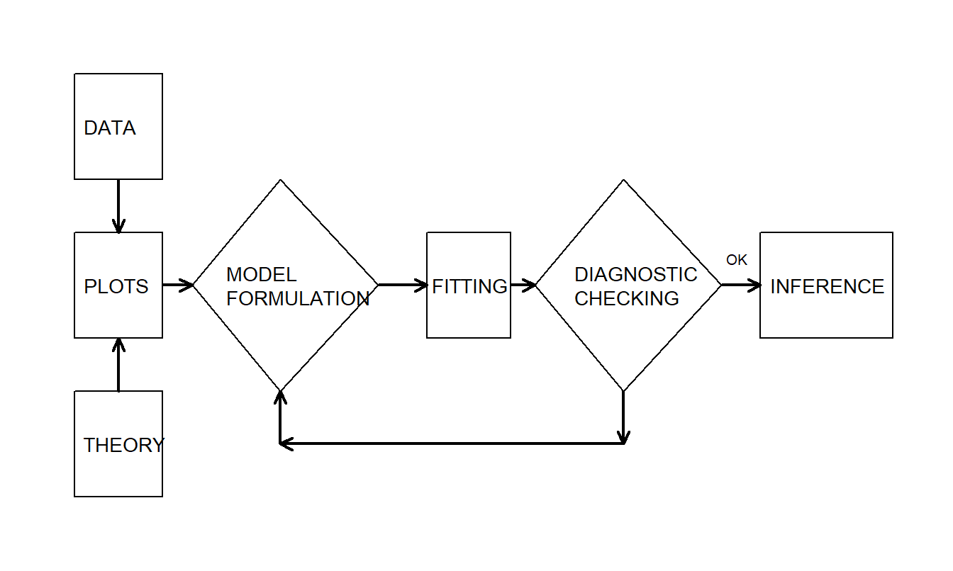
Figure 5.1: The iterative model specification process

This iterative process provides a useful recipe for structuring the task of specifying a model to represent a set of data. The first step, the model formulation stage, is accomplished by examining the data graphically and using prior knowledge of relationships, such as from economic theory or standard industry practice. The second step in the iteration is based on the assumptions of the specified model. These assumptions must be consistent with the data to make valid use of the model. The third step, diagnostic checking, is also known as data and model criticism; the data and model must be consistent with one another before additional inferences can be made. Diagnostic checking is an important part of the model formulation; it can reveal mistakes made in previous steps and provide ways to correct these mistakes.

Video: Section Summary

5.2 Automatic Variable Selection Procedures

Business and economics relationships are complicated; there are typically many variables that could serve as useful predictors of the dependent variable. In searching for a suitable relationship, there is a large number of potential models that are based on linear combinations of explanatory variables and an infinite number that can be formed from nonlinear combinations. To search among models based on linear combinations, several automatic procedures are available to select variables to be included in the model. These automatic procedures are easy to use and will suggest one or more models that you can explore in further detail.

To illustrate how large is the potential number of linear models, suppose that there are only four variables, f\(x_{1},\) \(x_2,\) \(x_3\) and \(x_4\), under consideration for fitting a model to \(y\). Without any consideration of multiplication or other nonlinear combinations of explanatory variables, how many possible models are there? Table 5.1 shows that the answer is 16.

Table 5.1: Sixteen Possible Models

Expression	Combinations	Models
E \(y=\beta_0\)		1 model with no independent variables
E \(y=\beta_0+\beta_1x_i\)	\(i\) = 1,2,3,4	4 models with one independent variable
E \(y = \beta_0 + \beta_1 x_i + \beta_2 x_j\)	(\(i,j\)) = (1,2),(1,3),(1,4),(2,3),(2,4),(3,4)	6 models with two independent variables
E \(y = \beta_0 + \beta_1 x_1 + \beta_2 x_j +\beta_3x_{k}\)	(\(i,j,k\)) = (1,2,3),(1,2,4),(1,3,4),(2,3,4)	4 models with three independent variables
E \(y = \beta_0 + \beta_1 x_1 + \beta_2 x_2 +\beta_3 x_3 + \beta_4 x_4\)		1 model with all independent variables

If there were only three explanatory variables, then you can use the same logic to verify that there are eight possible models. Extrapolating from these two examples, how many linear models will there be if there are ten explanatory variables? The answer is 1,024, which is quite a few. In general, the answer is \(2^k\), where \(k\) is the number of explanatory variables. For example, \(2^3\) is 8, \(2^4\) is 16, and so on.

In any case, for a moderately large number of explanatory variables, there are many potential models that are based on linear combinations of explanatory variables. We would like a procedure to search quickly through these potential models to give us more time to think about other interesting aspects of model selection. Stepwise regression are procedures that employ \(t\)-tests to check the “significance” of explanatory variables entered into, or deleted from, the model.

To begin, in the forward selection version of stepwise regression, variables are added one at a time. In the first stage, out of all the candidate variables the one that is most statistically significant is added to the model. At the next stage, with the first stage variable already included, the next most statistically significant variable is added. This procedure is repeated until all statistically significant variables have been added. Here, statistical significance is typically assessed using a variable’s \(t\)-ratio – the cut-off for statistical significance is typically a pre-determined \(t\)-value (such as two, corresponding to an approximate 95% significance level).

The backwards selection version works in a similar manner, except that all variables are included in the initial stage and then are dropped one at a time (instead of added).

More generally, an algorithm that adds and deletes variables at each stage is sometimes known as the stepwise regression algorithm.

Stepwise Regression Algorithm. Suppose that the analyst has identified one variable as the response, \(y\), and \(k\) potential explanatory variables, \(x_1, x_2, \ldots, x_k\).

1. Consider all possible regressions using one explanatory variable. For each of the \(k\) regressions, compute \(t(b_1)\), the \(t\)-ratio for the slope. Choose that variable with the largest \(t\)-ratio. If the \(t\)-ratio does not exceed a pre-specified \(t\)-value (such as two), then do not choose any variables and halt the procedure.
2. Add a variable to the model from the previous step. The variable to enter is the one that makes the largest significant contribution. To determine the size of contribution, use the absolute value of the variable’s \(t\)-ratio. To enter, the \(t\)-ratio must exceed a specified \(t\)-value in absolute value.
3. Delete a variable from the model in the previous step. The variable to be removed is the one that makes the smallest contribution. To determine the size of contribution, use the absolute value of the variable’s \(t\)-ratio. To be removed, the \(t\)-ratio must be less than a specified \(t\)-value in absolute value.
4. Repeat steps (ii) and (iii) until all possible additions and deletions are performed.

When implementing this routine, some statistical software packages use an \(F\)-test in lieu of \(t\)-tests. Recall, when only one variable is being considered, that \((t\text{-ratio})^2 = F\)-ratio and thus these procedures are equivalent.

This algorithm is useful in that it quickly searches through a number of candidate models. However, there are several drawbacks:

1. The procedure “snoops” through a large number of models and may fit the data “too well.”
2. There is no guarantee that the selected model is the best. The algorithm does not consider models that are based on nonlinear combinations of explanatory variables. It also ignores the presence of outliers and high leverage points.
3. In addition, the algorithm does not even search all \(2^{k}\) possible linear regressions.
4. The algorithm uses one criterion, a \(t\)-ratio, and does not consider other criteria such as \(s\), \(R^2\), \(R_a^2\), and so on.
5. There is a sequence of significance tests involved. Thus, the significance level that determines the \(t\)-value is not meaningful.
6. By considering each variable separately, the algorithm does not take into account the joint effect of explanatory variables.
7. Purely automatic procedures may not take into account an investigator’s special knowledge.

Many of the criticisms of the basic stepwise regression algorithm can be addressed with modern computing software that is now widely available. We now consider each drawback, in reverse order. To respond to drawback number (7), many statistical software routines have options for forcing variables into a model equation. In this way, if other evidence indicates that one or more variables should be included in the model, then the investigator can force the inclusion of these variables.

For drawback number (6), in Section 5.5.4 on suppressor variables, we will provide examples of variables that do not have important individual effects but are important when considered jointly. These combinations of variables may not be detected with the basic algorithm but will be detected with the backwards selection algorithm. Because the backwards procedure starts with all variables, it will detect, and retain, variables that are jointly important.

Drawback number (5) is really a suggestion about the way to use stepwise regression. Bendel and Afifi (1977) suggested using a cut-off smaller than you ordinarily might. For example, in lieu of using \(t\)-value = 2 corresponding approximately to a 5% significance level, consider using \(t\)-value = 1.645 corresponding approximately to a 10% significance level. In this way, there is less chance of screening out variables that may be important. A lower bound, but still a good choice for exploratory work, is a cut-off as small as \(t\)-value = 1. This choice is motivated by an algebraic result: when a variable enters a model, \(s\) will decrease if the \(t\)-ratio exceeds one in absolute value.

To address drawbacks number (3) and (4), we now introduce the best regressions routine. Best regressions is a useful algorithm that is now widely available in statistical software packages. The best regression algorithm searches over all possible combinations of explanatory variables, unlike stepwise regression, that adds and deletes one variable at a time. For example, suppose that there are four possible explanatory variables, \(x_1\), \(x_2\), \(x_3\), and \(x_4\), and the user would like to know what is the best two-variable model. The best regression algorithm searches over all six models of the form \(\mathrm{E}~y = \beta_0 + \beta_1 x_i + \beta_2 x_j\). Typically, a best regression routine recommends one or two models for each \(p\) coefficient model, where p is a number that is user-specified. Because it has specified the number of coefficients to enter the model, it does not matter which of the criteria we use: \(R^2\), \(R_a^2\), or \(s\).

The best regression algorithm performs its search by a clever use of the algebraic fact that, when a variable is added to the model, the error sum of squares does not increase. Because of this fact, certain combinations of variables included in the model need not be computed. An important drawback of this algorithm is that it can take a considerable amount of time when the number of variables considered is large.

Users of regression do not always appreciate the depth of drawback number (1), data-snooping. Data-snooping occurs when the analyst fits a great number of models to a data set. We will address the problem of data-snooping in Section 5.6.2 on model validation. Here, we illustrate the effect of data-snooping in stepwise regression.

---

Example: Data-Snooping in Stepwise Regression. The idea of this illustration is due to Rencher and Pun (1980). Consider \(n = 100\) observations of \(y\) and fifty explanatory variables, \(x_1, x_2, \ldots, x_{50}\). The data we consider here were simulated using independent standard normal random variates. Because the variables were simulated independently, we are working under the null hypothesis of no relation between the response and the explanatory variables, that is, \(H_0: \beta_1 = \beta_2 = \ldots = \beta_{50} = 0\). Indeed, when the model with all fifty explanatory variables was fit, it turns out that \(s = 1.142\), \(R^2 = 46.2\%\), and \(F\)-ratio = \(\frac{Regression~MS}{Error~MS} = 0.84\). Using an \(F\)-distribution with \(df_1 = 50\) and \(df_2 = 49\), the 95th percentile is 1.604. In fact, 0.84 is the 27th percentile of this distribution, indicating that the \(p\)-value is 0.73. Thus, as expected, the data are in congruence with \(H_0\).

Next, a stepwise regression with \(t\)-value = 2 was performed. Two variables were retained by this procedure, yielding a model with \(s = 1.05\), \(R^2 = 9.5\%\), and \(F\)-ratio = 5.09. For an \(F\)-distribution with \(df_1 = 2\) and \(df_2 = 97\), the 95th percentile is \(F\)-value = 3.09. This indicates that the two variables are statistically significant predictors of \(y\). At first glance, this result is surprising. The data were generated so that \(y\) is unrelated to the explanatory variables. However, because \(F\)-ratio \(>\) \(F\)-value, the \(F\)-test indicates that two explanatory variables are significantly related to \(y\). The reason is that stepwise regression has performed many hypothesis tests on the data. For example, in Step 1, fifty tests were performed to find significant variables. Recall that a 5% level means that we expect to make roughly one mistake in 20. Thus, with fifty tests, we expect to find \(50 \times 0.05 = 2.5\) “significant” variables, even under the null hypothesis of no relationship between \(y\) and the explanatory variables.

To continue, a stepwise regression with \(t\)-value = 1.645 was performed. Six variables were retained by this procedure, yielding a model with \(s = 0.99\), \(R^2 = 22.9\%\), and \(F\)-ratio = 4.61. As before, an \(F\)-test indicates a significant relationship between the response and these six explanatory variables.

To summarize, using simulation we constructed a data set so that the explanatory variables have no relationship with the response. However, when using stepwise regression to examine the data, we “found” seemingly significant relationships between the response and certain subsets of the explanatory variables. This example illustrates a general caveat in model selection: when explanatory variables are selected using the data, \(t\)-ratios and \(F\)-ratios will be too large, thus overstating the importance of variables in the model.

---

Stepwise regression and best regressions are examples of automatic variable selection procedures. In your modeling work, you will find these procedures to be useful because they can quickly search through several candidate models. However, these procedures do ignore nonlinear alternatives as well as the effect of outliers and high leverage points. The main point of the procedures is to mechanize certain routine tasks. This automatic selection approach can be extended and indeed, there are a number of so-called “expert systems” available in the market. For example, algorithms are available that “automatically” handle unusual points such as outliers and high leverage points. A model suggested by automatic variable selection procedures should be subject to the same careful diagnostic checking procedures as a model arrived at by any other means.

Video: Section Summary

5.3 Residual Analysis

Recall the role of a residual in the linear regression model introduced in Section 2.6. A residual is a response minus the corresponding fitted value under the model. Because the model summarizes the linear effect of several explanatory variables, we may think of a residual as a response controlled for values of the explanatory variables. If the model is an adequate representation of the data, then residuals should closely approximate random errors. Random errors are used to represent the natural variation in the model; they represent the result of an unpredictable mechanism. Thus, to the extent that residuals resemble random errors, there should be no discernible patterns in the residuals. Patterns in the residuals indicate the presence of additional information that we hope to incorporate into the model. A lack of patterns in the residuals indicates that the model seems to account for the primary relationships in the data.

5.3.1 Residuals

There are at least four types of patterns that can be uncovered through the residual analysis. In this section, we discuss the first two: residuals that are unusual and those that are related to other explanatory variables. We then introduce the third type, residuals that display a heteroscedastic pattern, in Section 5.7. In our study of time series data that begins in Chapter 7, we will introduce the fourth type, residuals that display patterns through time.

When examining residuals, it is usually easier to work with a standardized residual, a residual that has been rescaled to be dimensionless. We generally work with standardized residuals because we achieve some carry-over of experience from one data set to another and may thus focus on relationships of interest. By using standardized residuals, we can train ourselves to look at a variety of residual plots and immediately recognize an unusual point when working in standard units.

There are a number of ways of defining a standardized residual. Using \(e_i = y_i - \hat{y}_i\) as the \(i\)th residual, here are three commonly used definitions:

\[\begin{equation} \text{(a) }\frac{e_i}{s}, \quad \text{(b) }\frac{e_i}{s\sqrt{1 - h_{ii}}}, \quad \text{(c) }\frac{e_i}{s_{(i)}\sqrt{1 - h_{ii}}}. \tag{5.1} \end{equation}\]

Here, \(h_{ii}\) is the \(i\)th leverage. It is calculated based on values of the explanatory variables and will be defined in Section 5.4.1. Recall that \(s\) is the residual standard deviation (defined in equation 3.8). Similarly, define \(s_{(i)}\) to be the residual standard deviation when running a regression after having deleted the \(i\)th observation.

Now, the first definition in (a) is simple and easy to explain. An easy calculation shows that the sample standard deviation of the residuals is approximately \(s\) (one reason that \(s\) is often referred to as the residual standard deviation). Thus, it seems reasonable to standardize residuals by dividing by \(s\).

The second choice presented in (b), although more complex, is more precise. The variance of the \(i\)th residual is

\[ \text{Var}(e_i) = \sigma^2(1 - h_{ii}). \]

This result will be established in equation (5.15) of Section 5.10. Note that this variance is smaller than the variance of the error term, Var\((\varepsilon_i) = \sigma^2\). Now, we can replace \(\sigma\) by its estimate, \(s\). Then, this result leads to using the quantity \(s\sqrt{1 - h_{ii}}\) as an estimated standard deviation, or standard error, for \(e_i\). Thus, we define the standard error of \(e_i\) to be

\[ \text{se}(e_i) = s \sqrt{1 - h_{ii}}. \]

Following the conventions introduced in Section 2.6, in this text we use \(e_i / \text{se}(e_i)\) to be our standardized residual.

The third choice presented in (c) is a modification of (b) and is known as a studentized residual. As emphasized in Section 5.3.2, one important use of residuals is to identify unusually large responses. Now, suppose that the \(i\)th response is unusually large and that this is measured through its residual. This unusually large residual will also cause the value of \(s\) to be large. Because the large effect appears in both the numerator and denominator, the standardized residual may not detect this unusual response. However, this large response will not inflate \(s_{(i)}\) because it is constructed after having deleted the \(i\)th observation. Thus, when using studentized residuals, we get a better measure of observations that have unusually large residuals. By omitting this observation from the estimate of \(\sigma\), the size of the observation affects only the numerator \(e_i\) and not the denominator \(s_{(i)}\).

As another advantage, studentized residuals follow a \(t\)-distribution with \(n - (k + 1)\) degrees of freedom, assuming the errors are normally distributed (assumption E5). This knowledge of the precise distribution helps us assess the degree of model fit and is particularly useful in small samples. It is this relationship with the “Student’s” \(t\)-distribution that suggests the name “studentized” residuals.

5.3.2 Using Residuals to Identify Outliers

One important role of residual analysis is to identify outliers. An outlier is an observation that is not well fit by the model; these are observations where the residual is unusually large. A rule of thumb that is used by many statistical packages is that an observation is marked as an outlier if the standardized residual exceeds two in absolute value. To the extent that the distribution of standardized residuals mimics the standard normal curve, we expect about only one in 20 observations, or 95%, to exceed two in absolute value and very few observations to exceed three.

Outliers provide a signal that an observation should be investigated to understand special causes associated with this point. An outlier is an observation that seems unusual with respect to the rest of the data set. It is often the case that the reason for this atypical behavior may be uncovered after additional investigation. Indeed, this may be the primary purpose of the regression analysis of a data set.

Consider a simple example of so-called performance analysis. Suppose we have available a sample of \(n\) salespeople and are trying to understand each person’s second-year sales based on their first-year sales. To a certain extent, we expect that higher first-year sales are associated with higher second-year sales. High sales may be due to a salesperson’s natural ability, ambition, good territory, and so on. First-year sales may be thought of as a proxy variable that summarizes these factors. We expect variation in sales performance both cross-sectionally and across years. It is interesting when one salesperson performs unusually well (or poorly) in the second year compared to their first-year performance. Residuals provide a formal mechanism for evaluating second-year sales after controlling for the effects of first-year sales.

There are a number of options available for handling outliers.

Options for Handling Outliers

• Include the observation in the usual summary statistics but comment on its effects. An outlier may be large but not so large as to skew the results of the entire analysis. If no special causes for this unusual observation can be determined, then this observation may simply reflect the variability in the data.
• Delete the observation from the data set. The observation may be determined to be unrepresentative of the population from which the sample is drawn. If this is the case, then there may be little information contained in the observation that can be used to make general statements about the population. This option means that we would omit the observation from the regression summary statistics and discuss it in our report as a separate case.
• Create a binary variable to indicate the presence of an outlier. If one or several special causes have been identified to explain an outlier, then these causes could be introduced into the modeling procedure formally by introducing a variable to indicate the presence (or absence) of these causes. This approach is similar to point deletion but allows the outlier to be formally included in the model formulation so that, if additional observations arise that are affected by the same causes, then they can be handled on an automatic basis.

5.3.3 Using Residuals to Select Explanatory Variables

Another important role of residual analysis is to help identify additional explanatory variables that may be used to improve the formulation of the model. If we have specified the model correctly, then residuals should resemble random errors and contain no discernible patterns. Thus, when comparing residuals to explanatory variables, we do not expect any relationships. If we do detect a relationship, then this suggests the need to control for this additional variable. This can be accomplished by introducing the additional variable into the regression model.

Relationships between residuals and explanatory variables can be quickly established using correlation statistics. However, if an explanatory variable is already included in the regression model, then the correlation between the residuals and an explanatory variable will be zero (see Section 5.10.1 for the algebraic demonstration). It is a good idea to reinforce this correlation with a scatter plot. Not only will a plot of residuals versus explanatory variables reinforce graphically the correlation statistic, it will also serve to detect potential nonlinear relationships. For example, a quadratic relationship can be detected using a scatter plot, not a correlation statistic.

If you detect a relationship between the residuals from a preliminary model fit and an additional explanatory variable, then introducing this additional variable will not always improve your model specification. The reason is that the additional variable may be linearly related to the variables that are already in the model. If you would like a guarantee that adding an additional variable will improve your model, then construct an added variable plot (see Section 3.4.3).

To summarize, after a preliminary model fit, you should:

• Calculate summary statistics and display the distribution of (standardized) residuals to identify outliers.
• Calculate the correlation between the (standardized) residuals and additional explanatory variables to search for linear relationships.
• Create scatter plots between the (standardized) residuals and additional explanatory variables to search for nonlinear relationships.

---

Example: Stock Market Liquidity. An investor’s decision to purchase a stock is generally made with a number of criteria in mind. First, investors usually look for a high expected return. A second criterion is the riskiness of a stock, which can be measured through the variability of the returns. Third, many investors are concerned with the length of time that they are committing their capital with the purchase of a security. Many income stocks, such as utilities, regularly return portions of capital investments in the form of dividends. Other stocks, particularly growth stocks, return nothing until the sale of the security. Thus, the average length of investment in a security is another criterion. Fourth, investors are concerned with the ability to sell the stock at any time convenient to the investor. We refer to this fourth criterion as the liquidity of the stock. The more liquid the stock, the easier it is to sell. To measure liquidity, in this study we use the number of shares traded on an exchange over a specified period of time (called the VOLUME). We are interested in studying the relationship between the volume and other financial characteristics of a stock.

We begin this study with 126 companies whose options were traded on December 3, 1984. The stock data were obtained from Francis Emory Fitch, Inc. for the period from December 3, 1984 to February 28, 1985. For the trading activity variables, we examine:

• The three months total trading volume (VOLUME, in millions of shares),
• The three months total number of transactions (NTRAN), and
• The average time between transactions (AVGT, measured in minutes).

For the firm size variables, we use:

• Opening stock price on January 2, 1985 (PRICE),
• The number of outstanding shares on December 31, 1984 (SHARE, in millions of shares), and
• The market equity value (VALUE, in billions of dollars) obtained by taking the product of PRICE and SHARE.

Finally, for the financial leverage, we examine the debt-to-equity ratio (DEB_EQ) obtained from the Compustat Industrial Tape and the Moody’s manual. The data in SHARE are obtained from the Center for Research in Security Prices (CRSP) monthly tape.

After examining some preliminary summary statistics of the data, three companies were deleted because they either had an unusually large volume or high price. They are Teledyne and Capital Cities Communication, whose prices were more than four times the average price of the remaining companies, and American Telephone and Telegraph, whose total volume was more than seven times the average total volume of the remaining companies. Based on additional investigation, the details of which are not presented here, these companies were deleted because they seemed to represent special circumstances that we would not wish to model.

Table 5.2 summarizes the descriptive statistics based on the remaining \(n = 123\) companies. For example, from Table 5.2, we see that the average time between transactions is about five minutes and this time ranges from a minimum of less than 1 minute to a maximum of about 20 minutes.

Table 5.2: Summary Statistics of the Stock Liquidity Variables

	Mean	Median	Standard Deviation	Minimum	Maximum
VOLUME	13.423	11.556	10.632	0.658	64.572
AVGT	5.441	4.284	3.853	0.590	20.772
NTRAN	6436.000	5071.000	5310.000	999.000	36420.000
PRICE	38.800	34.380	21.370	9.120	122.380
SHARE	94.730	53.830	115.100	6.740	783.050
VALUE	4.116	2.065	8.157	0.115	75.437
DEBEQ	2.697	1.105	6.509	0.185	53.628

Source: Francis Emory Fitch, Inc., Standard & Poor’s Compustat, and University of Chicago’s Center for Research on Security Prices.

Table 5.3 reports the correlation coefficients and Figure 5.2 provides the corresponding scatterplot matrix. If you have a background in finance, you will find it interesting to note that the financial leverage, measured by DEB_EQ, does not seem to be related to the other variables. From the scatterplot and correlation matrix, we see a strong relationship between VOLUME and the size of the firm as measured by SHARE and VALUE. Further, the three trading activity variables, VOLUME, AVGT, and NTRAN, are all highly related to one another.

Table 5.3: Correlation Matrix of the Stock Liquidity

	AVGT	NTRAN	PRICE	SHARE	VALUE	DEB_EQ	VOLUME
AVGT	1.000	-0.668	-0.128	-0.429	-0.318	0.094	-0.674
NTRAN	-0.668	1.000	0.190	0.817	0.760	-0.092	0.913
PRICE	-0.128	0.190	1.000	0.177	0.457	-0.038	0.168
SHARE	-0.429	0.817	0.177	1.000	0.829	-0.077	0.773
VALUE	-0.318	0.760	0.457	0.829	1.000	-0.077	0.702
DEB_EQ	0.094	-0.092	-0.038	-0.077	-0.077	1.000	-0.052
VOLUME	-0.674	0.913	0.168	0.773	0.702	-0.052	1.000

R Code to Produce Tables 5.2 and 5.3

liquidity <- read.csv("CSVData/Liquidity.csv", header=TRUE)
varLiquid <- c("AVGT", "NTRAN", "PRICE", "SHARE", "VALUE", "DEBEQ", "VOLUME")
liquidMat <- data.frame(liquidity[varLiquid])
names(liquidMat)[names(liquidMat) == "DEBEQ"] <- "DEB_EQ"

#  TABLE 5.2 SUMMARY STATISTICS
BookSummStats <- function(Xymat){
meanSummary <- sapply(Xymat, mean,  na.rm=TRUE) 
sdSummary   <- sapply(Xymat, sd,    na.rm=TRUE) 
minSummary  <- sapply(Xymat, min,   na.rm=TRUE) 
maxSummary  <- sapply(Xymat, max,   na.rm=TRUE) 
medSummary  <- sapply(Xymat, median,na.rm=TRUE) 
tableMat  <- cbind(meanSummary, medSummary, sdSummary, minSummary, maxSummary)
return(tableMat)
}

liquidMat1 <- liquidMat[,c(7,1:6)]
tableMat  <- BookSummStats(liquidMat1)
colnames(tableMat)  <- c("Mean" , "Median" , "Standard Deviation" , 
                         "Minimum" , "Maximum")
rownames(tableMat)  <- varLiquid[c(7,1:6)]
tableMat       <- round(tableMat, digits = 3)
tableMat[3,]   <- round(tableMat[3,], digits = 0) 
tableMat[4:5,] <- round(tableMat[4:5,], digits = 2)

TableGen1(TableData=tableMat, 
         TextTitle='Summary Statistics of the Stock Liquidity Variables', 
         Align='r', Digits=3, ColumnSpec=1:5,
         ColWidth = ColWidth5) 

cor_matrix <- cor(liquidMat)
rownames(cor_matrix) <- colnames(cor_matrix) <- 
        c("AVGT", "NTRAN", "PRICE", "SHARE", "VALUE", "DEB_EQ", "VOLUME")
TableGen1(TableData=cor_matrix, 
         TextTitle='Correlation Matrix of the Stock Liquidity', 
         Align='r', Digits=3, ColumnSpec=1:6,
         ColWidth = ColWidth6) 

Figure 5.2 shows that the variable AVGT is inversely related to VOLUME and NTRAN is inversely related to AVGT. In fact, it turned out the correlation between the average time between transactions and the reciprocal of the number of transactions was \(99.98\%!\) This is not so surprising when one thinks about how AVGT might be calculated. For example, on the New York Stock Exchange, the market is open from 10:00 A.M. to 4:00 P.M. For each stock on a particular day, the average time between transactions times the number of transactions is nearly equal to 360 minutes (= 6 hours). Thus, except for rounding errors because transactions are only recorded to the nearest minute, there is a perfect linear relationship between AVGT and the reciprocal of NTRAN.

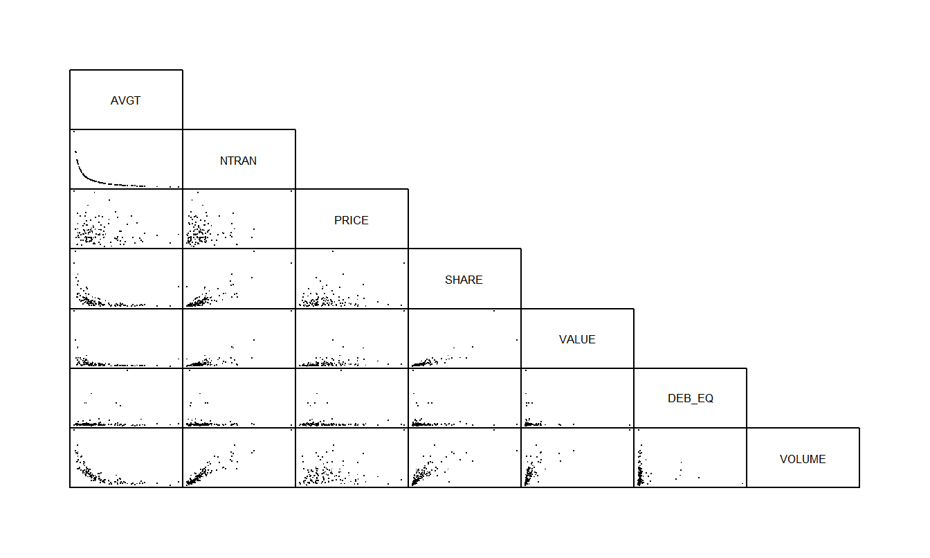
Figure 5.2: Scatterplot matrix for stock liquidity variables. The number of transactions variable (NTRAN) appears to be strongly related to the VOLUME of shares traded, and inversely related to AVGT.

To begin to understand the liquidity measure VOLUME, we first fit a regression model using NTRAN as an explanatory variable. The fitted regression model is:

\[ \small{ \begin{array}{lcc} \text{VOLUME} &= 1.65 &+ 0.00183 \text{ NTRAN} \\ \text{standard errors} & (0.6173) & (0.000074) \end{array} } \]

with \(R^2 = 83.4\%\) and \(s = 4.35\). Note that the \(t\)-ratio for the slope associated with NTRAN is

\[ t(b_1) = \frac{b_1}{se(b_1)} = \frac{0.00183}{0.000074} = 24.7 \]

indicating strong statistical significance. Residuals were computed using this estimated model. To see if the residuals are related to the other explanatory variables, Table 5.4 shows correlations.

Table 5.4: First Table of Correlations

Variable	AVGT	PRICE	SHARE	VALUE	DEB_EQ
RESID	-0.159	-0.014	0.064	0.018	0.078

Note: The residuals were created from a regression of VOLUME on NTRAN.

The correlation between the residual and AVGT and the scatter plot (not shown here) indicates that there may be some information in the variable AVGT in the residual. Thus, it seems sensible to use AVGT directly in the regression model. Remember that we are interpreting the residual as the value of VOLUME having controlled for the effect of NTRAN.

We next fit a regression model using NTRAN and AVGT as explanatory variables. The fitted regression model is:

\[ \small{ \begin{array}{lccc} \text{VOLUME} &= 4.41 &- 0.322 \text{ AVGT} &+ 0.00167 \text{ NTRAN} \\ \text{standard errors} & (1.30)& (0.135)& (0.000098) \end{array} } \]

with \(R^2 = 84.2\%\) and \(s = 4.26\). Based on the \(t\)-ratio for AVGT, \(t(b_{AVGT}) = \frac{-0.322}{0.135} = -2.39\), it seems as if AVGT is a useful explanatory variable in the model. Note also that \(s\) has decreased, indicating that \(R_a^2\) has increased.

Table 5.5 provides correlations between the model residuals and other potential explanatory variables and indicates that there does not seem to be much additional information in the explanatory variables. This is reaffirmed by the corresponding table of scatter plots in Figure 5.3. The histograms in Figure 5.3 suggest that although the distribution of the residuals is fairly symmetric, the distribution of each explanatory variable is skewed. Because of this, transformations of the explanatory variables were explored. This line of thought provided no real improvements and thus the details are not provided here.

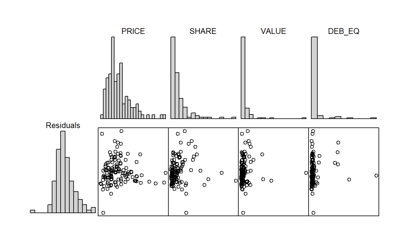
Figure 5.3: Scatterplot matrix of the residuals from the regression of VOLUME on NTRAN and AVGT on the vertical axis and the remaining predictor variables on the horizontal axes.

Table 5.5: Second Table of Correlations

Variable	PRICE	SHARE	VALUE	DEB_EQ
RESID	-0.015	0.100	0.074	0.089

Note: The residuals were created from a regression of VOLUME on NTRAN and AVGT.

Video: Section Summary

5.4 Influential Points

Not all points are created equal – in this section we will see that specific observations can potentially have a disproportionate effect on the overall regression fit. We will call such points “influential.” This is not too surprising; we have already seen that regression coefficient estimates are weighted sums of responses (see Section 3.2.4). Some observations have heavier weights than others and thus have a greater influence on the regression coefficient estimates. Of course, simply because an observation is influential does not mean that it is incorrect or that its impact on the model is misleading. As analysts, we would simply like to know whether our fitted model is sensitive to mild changes such as the removal of a single point so that we feel comfortable generalizing our results from the sample to a larger population.

To assess influence, we think of observations as being unusual responses, given a set of explanatory variables, or having an unusual set of explanatory variables values. We have already seen in Section 5.3 how to assess unusual responses using residuals. This section focuses on unusual sets of explanatory variables values.

5.4.1 Leverage

We introduced this topic in Section 2.6 where we called an observation having an unusual explanatory variable value a “high leverage point.” With more than one explanatory variable, determining whether an observation is a high leverage point is not as straightforward. For example, it is possible for an observation to be “not unusual” for any single variable and yet still be unusual in the space of explanatory variables. Consider the fictitious data set represented in Figure 5.4. Visually, it seems clear that the point marked in the upper right-hand corner is unusual. However, it is not unusual when examining the histogram of either \(x_1\) or \(x_2\). It is only unusual when the explanatory variables are considered jointly.

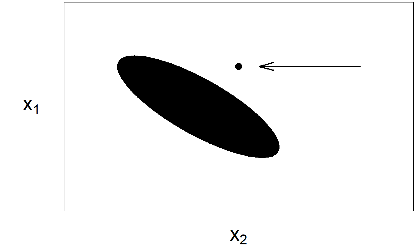
Figure 5.4: The ellipsoid represents most of the data. The arrow marks an unusual point.

For two explanatory variables, this is apparent when examining the data graphically. Because it is difficult to examine graphically data having more than two explanatory variables, we need a numerical procedure for assessing leverage.

To define the concept of leverage in multiple linear regression, we use some concepts from matrix algebra. Specifically, in Section 3.1, we showed that the vector of least squares regression coefficients could be calculated using \(\mathbf{b} = (\mathbf{X}^{\prime} \mathbf{X})^{-1} \mathbf{X}^{\prime} \mathbf{y}\). Thus, we can express the vector of fitted values \(\hat{\mathbf{y}} = (\hat{y}_1, \ldots, \hat{y}_n)^{\prime}\) as

\[\begin{equation} \mathbf{\hat{y}} = \mathbf{Xb} . \tag{5.2} \end{equation}\]

Similarly, the vector of residuals is the vector of response minus the vector of fitted values, that is, \(\mathbf{e} = \mathbf{y - \hat{y}}\).

From the expression for the regression coefficients \(\mathbf{b}\) in equation (3.4), we have

\[ \mathbf{\hat{y}} = \mathbf{X} (\mathbf{X}^{\prime} \mathbf{X})^{-1} \mathbf{X}^{\prime} \mathbf{y} \]

This equation suggests defining

\[ \mathbf{H} = \mathbf{X} (\mathbf{X}^{\prime} \mathbf{X})^{-1} \mathbf{X}^{\prime} \]

so that

\[ \mathbf{\hat{y}} = \mathbf{Hy} \]

From this, the matrix \(\mathbf{H}\) is said to project the vector of responses \(\mathbf{y}\) onto the vector of fitted values \(\mathbf{\hat{y}}\). Alternatively, you may think of \(\mathbf{H}\) as the matrix that puts the “hat,” or carat, on \(\mathbf{y}\). From the \(i\)th row of the vector equation \(\mathbf{\hat{y}} = \mathbf{Hy}\), we have

\[ \hat{y}_i = h_{i1} y_1 + h_{i2} y_2 + \cdots + h_{ii} y_i + \cdots + h_{in} y_n \]

Here, \(h_{ij}\) is the number in the \(i\)th row and \(j\)th column of \(\mathbf{H}\). From this expression, we see that the larger \(h_{ii}\) is, the larger the effect that the \(i\)th response \((y_i)\) has on the corresponding fitted value \((\hat{y}_i)\). Thus, we call \(h_{ii}\) the leverage for the \(i\)th observation. Because \(h_{ii}\) is the \(i\)th diagonal element of \(\mathbf{H}\), a direct expression for \(h_{ii}\) is

\[\begin{equation} h_{ii} = \mathbf{x}_i^{\prime} (\mathbf{X}^{\prime} \mathbf{X})^{-1} \mathbf{x}_i \tag{5.3} \end{equation}\]

where \(\mathbf{x}_i = (x_{i0}, x_{i1}, \ldots, x_{ik})^{\prime}\). Because the values \(h_{ii}\) are calculated based on the explanatory variables, the values of the response variable do not affect the calculation of leverages.

Large leverage values indicate that an observation may exhibit a disproportionate effect on the fit, essentially because it is distant from the other observations (when looking at the space of explanatory variables). How large is large? Some guidelines are available from matrix algebra, where we have that

\[ \frac{1}{n} \le h_{ii} \le 1 \]

and

\[ \bar{h} = \frac{1}{n} \sum_{i=1}^{n} h_{ii} = \frac{k+1}{n}. \]

Thus, each leverage is bounded by \(n^{-1}\) and \(1\), and the average leverage equals the number of regression coefficients divided by the number of observations. From these and related arguments, we use a widely adopted convention and declare an observation to be a high leverage point if the leverage exceeds three times the average, that is, if

\[ h_{ii} > \frac{3(k+1)}{n}. \]

Having identified high leverage points, as with outliers it is important for the analyst to search for special causes that may have produced these unusual points. To illustrate, in Section 2.7 we identified the 1987 market crash as the reason behind the high leverage point. Further, high leverage points are often due to clerical errors in coding the data, which may or may not be easy to rectify. In general, the options for dealing with high leverage points are similar to those available for dealing with outliers.

Options for Handling High Leverage Points

1. Include the observation in the summary statistics but comment on its effect. For example, an observation may barely exceed a cut-off and its effect may not be important in the overall analysis.
2. Delete the observation from the data set. Again, the basic rationale for this action is that the observation is deemed not representative of some larger population. An intermediate course of action between (1) and (2) is to present the analysis both with and without the high leverage point. In this way, the impact of the point is fully demonstrated and the reader of your analysis may decide which option is more appropriate.
3. Choose another variable to represent the information. In some instances, another explanatory variable will be available to serve as a replacement. For example, in an apartment rents example, we could use the number of bedrooms to replace a square footage variable as a measure of apartment size. Although an apartment’s square footage may be unusually large causing it to be a high leverage point, it may have one, two, or three bedrooms, depending on the sample examined.
4. Use a nonlinear transformation of an explanatory variable. To illustrate, with our Stock Liquidity example in Section 5.5.3, we can transform the debt-to-equity DEB_EQ continuous variable into a variable that indicates the presence of “high” debt-to-equity. For example, we might code DE_IND = 1 if DEB_EQ > 5 and DE_IND = 0 if DEB_EQ ≤ 5. With this recoding, we still retain information on the financial leverage of a company without allowing the large values of DEB_EQ to drive the regression fit.

Some analysts use “robust” estimation methodologies as an alternative to least squares estimation. The basic idea of these techniques is to reduce the effect of any particular observation. These techniques are useful in reducing the effect of both outliers and high leverage points. This tactic may be viewed as intermediate between one extreme procedure, ignoring the effect of unusual points, and another extreme, giving unusual points full credibility by deleting them from the data set. The word robust is meant to suggest that these estimation methodologies are “healthy” even when attacked by an occasional bad observation (a germ). We have seen that this is not true for least squares estimation.

5.4.2 Cook’s Distance

To quantify the influence of a point, a measure that considers both the response and explanatory variables is Cook’s Distance. This distance, \(D_i\), is defined as

\[\begin{equation} \begin{array}{ll} D_i &= \frac{\sum_{j=1}^{n} (\hat{y}_j - \hat{y}_{j(i)})^2}{(k+1) s^2} \tag{5.4} \\ &= \left( \frac{e_i}{se(e_i)} \right)^2 \frac{h_{ii}}{(k+1)(1 - h_{ii})}. \end{array} \end{equation}\]

The first expression provides a definition. Here, \(\hat{y}_{j(i)}\) is the prediction of the \(j\)th observation, computed leaving the \(i\)th observation out of the regression fit. To measure the impact of the \(i\)th observation, we compare the fitted values with and without the \(i\)th observation. Each difference is then squared and summed over all observations to summarize the impact.

The second equation provides another interpretation of the distance \(D_i\). The first part, \(\left( \frac{e_i}{se(e_i)} \right)^2\), is the square of the \(i\)th standardized residual. The second part, \(\frac{h_{ii}}{(k+1)(1 - h_{ii})}\), is attributable solely to the leverage. Thus, the distance \(D_i\) is composed of a measure for outliers times a measure for leverage. In this way, Cook’s distance accounts for both the response and explanatory variables. Section 5.10.3 establishes the validity of equation (5.4).

To get an idea of the expected size of \(D_i\) for a point that is not unusual, recall that we expect the standardized residuals to be about one and the leverage \(h_{ii}\) to be about \(\frac{k+1}{n}\). Thus, we anticipate that \(D_i\) should be about \(\frac{1}{n}\). Another rule of thumb is to compare \(D_i\) to an \(F\)-distribution with \(df_1 = k+1\) and \(df_2 = n - (k+1)\) degrees of freedom. Values of \(D_i\) that are large compared to this distribution merit attention.

---

Example: Outliers and High Leverage Points - Continued. To illustrate, we return to our example in Section 2.6. In this example, we considered 19 “good,” or base, points plus each of the three types of unusual points, labeled A, B, and C. Table 5.6 summarizes the calculations.

Table 5.6: Measures of Three Types of Unusual Points

Observation	Standardized Residual \(e / se(e)\)	Leverage \(h\)	Cook’s Distance \(D\)
A	4.00	0.067	0.577
B	0.77	0.550	0.363
C	-4.01	0.550	9.832

As noted in Section 2.6, from the standardized residual column we see that both points A and C are outliers. To judge the size of the leverages, because there are \(n=20\) points, the leverages are bounded by 0.05 and 1.00 with the average leverage being \(\bar{h} = \frac{2}{20} = 0.10\). Using 0.3 (\(= 3 \times \bar{h}\)) as a cut-off, both points B and C are high leverage points. Note that their values are the same. This is because, from Figure 2.7, the values of the explanatory variables are the same and only the response variable has been changed. The column for Cook’s distance captures both types of unusual behavior. Because the typical value of \(D_i\) is \(\frac{1}{n}\) or 0.05, Cook’s distance provides one statistic to alert us to the fact that each point is unusual in one respect or another. In particular, point C has a very large \(D_i\), reflecting the fact that it is both an outlier and a high leverage point. The 95th percentile of an \(F\)-distribution with \(df_1 = 2\) and \(df_2 = 18\) is 3.555. The fact that point C has a value of \(D_i\) that well exceeds this cut-off indicates the substantial influence of this point.

Video: Section Summary

5.5 Collinearity

5.5.1 What is Collinearity?

Collinearity, or multicollinearity, occurs when one explanatory variable is, or nearly is, a linear combination of the other explanatory variables. Intuitively, with collinear data it is useful to think of explanatory variables as being highly correlated with one another. If an explanatory variable is collinear, then the question arises as to whether it is redundant, that is, whether the variable provides little additional information over and above the information in the other explanatory variables. The issues are: Is collinearity important? If so, how does it affect our model fit and how do we detect it? To address the first question, consider a somewhat pathological example.

---

Example: Perfectly Correlated Explanatory Variables. Joe Finance was asked to fit the model \(\mathrm{E} ~y = \beta_0 + \beta_1 x_1 + \beta_2 x_2\) to a data set. His resulting fitted model was \(\hat{y} = -87 + x_1 + 18 x_2.\) The data set under consideration is:

\[ \begin{array}{l|cccc} \hline i & 1 & 2 & 3 & 4 \\ \hline y_i & 23 & 83 & 63 & 103 \\ x_{i1} & 2 & 8 &6 & 10 \\ x_{i2} & 6 & 9 & 8 & 10 \\ \hline \end{array} \]

Joe checked the fit for each observation. Joe was very happy because he fit the data perfectly! For example, for the third observation the fitted value is \(\hat{y}_3 = -87 + 6 + 18 \times 8 = 63\) which is equal to the third response, \(y_3\). Because the response equals the fitted value, the residual is zero. You may check that this is true of each observation and thus the \(R^2\) turned out to be \(100\%\).

However, Jane Actuary came along and fit the model \(\hat{y} = -7 + 9 x_1 + 2 x_2.\) Jane performed the same careful checks that Joe did and also got a perfect fit (\(R^2 = 1\)). Who is right?

The answer is both and neither one. There are, in fact, an infinite number of fits. This is due to the perfect relationship \(x_2 = 5 + \frac{x_1}{2}\) between the two explanatory variables.

---

This example illustrates some important facts about collinearity.

Collinearity Facts

• Collinearity neither precludes us from getting good fits nor from making predictions of new observations. Note that in the above example we got perfect fits.
• Estimates of error variances and, therefore, tests of model adequacy, are still reliable.
• In cases of serious collinearity, standard errors of individual regression coefficients are larger than cases where, other things equal, serious collinearity does not exist. With large standard errors, individual regression coefficients may not be meaningful. Further, because a large standard error means that the corresponding \(t\)-ratio is small, it is difficult to detect the importance of a variable.

To detect collinearity, begin with a matrix of correlation coefficients of the explanatory variables. This matrix is simple to create, easy to interpret, and quickly captures linear relationships between pairs of variables. A scatterplot matrix provides a visual reinforcement of the summary statistics in the correlation matrix.

5.5.2 Variance Inflation Factors

Correlation and scatterplot matrices capture only relationships between pairs of variables. To capture more complex relationships among several variables, we introduce the variance inflation factor (VIF). To define a VIF, suppose that the set of explanatory variables is labeled \(x_1, x_2, \ldots, x_{k}\). Now, run the regression using \(x_j\) as the “response” and the other \(x\)’s (\(x_1, x_2, \ldots, x_{j-1}, x_{j+1}, \ldots, x_{k}\)) as the explanatory variables. Denote the coefficient of determination from this regression by \(R_j^2\). We interpret \(R_j = \sqrt{R_j^2}\) as the multiple correlation coefficient between \(x_j\) and linear combinations of the other \(x\)’s. From this coefficient of determination, we define the variance inflation factor

\[ VIF_j = \frac{1}{1 - R_j^2}, \text{ for } j = 1, 2, \ldots, k. \]

A larger \(R_j^2\) results in a larger \(VIF_j\); this means greater collinearity between \(x_j\) and the other \(x\)’s. Now, \(R_j^2\) alone is enough to capture the linear relationship of interest. However, we use \(VIF_j\) in lieu of \(R_j^2\) as our measure for collinearity because of the algebraic relationship

\[\begin{equation} se(b_j) = s \frac{\sqrt{VIF_j}}{s_{x_j} \sqrt{n - 1}}. \tag{5.5} \end{equation}\]

Here, \(se(b_j)\) and \(s\) are standard errors and residual standard deviation from a full regression fit of \(y\) on \(x_1, \ldots, x_{k}\). Further, \(s_{x_j} = \sqrt{(n - 1)^{-1} \sum_{i=1}^{n} (x_{ij} - \bar{x}_j)^2 }\) is the sample standard deviation of the \(j\)th variable \(x_j\). Section 5.10.3 provides a verification of equation (5.5).

Thus, a larger \(VIF_j\) results in a larger standard error associated with the \(j\)th slope, \(b_j\). Recall that \(se(b_j)\) is \(s\) times the square root of the \((j+1)\)st diagonal element of \((\mathbf{X}^{\prime} \mathbf{X})^{-1}\). The idea is that when collinearity occurs, the matrix \(\mathbf{X}^{\prime} \mathbf{X}\) has properties similar to the number zero. When we attempt to calculate the inverse of \(\mathbf{X}^{\prime} \mathbf{X}\), this is analogous to dividing by zero for scalar numbers. As a rule of thumb, when \(VIF_j\) exceeds 10 (which is equivalent to \(R_j^2 > 90\%\)), we say that severe collinearity exists. This may signal a need for action. Tolerance, defined as the reciprocal of the variance inflation factor, is another measure of collinearity used by some analysts.

For example, with \(k = 2\) explanatory variables in the model, then \(R_1^2\) is the squared correlation between the two explanatory variables, say \(r_{12}^2\). Then, from the equation above, we have that

\[ se(b_j) = s \left(s_{x_j} \sqrt{n - 1} \right)^{-1} \left(1 - r_{12}^2 \right)^{-1/2}, \text{ for } j = 1, 2. \]

As the correlation approaches one in absolute value, \(|r_{12}| \rightarrow 1\), then the standard error becomes large meaning that the corresponding \(t\)-statistic becomes small. In summary, a high \(VIF\) may mean small \(t\)-statistics even though variables are important. Further, one can check that the correlation between \(b_1\) and \(b_2\) is \(-r_{12}\), indicating that the coefficient estimates are highly correlated.

Example: Stock Market Liquidity - Continued. As an example, consider a regression of VOLUME on PRICE, SHARE, and VALUE. Unlike the explanatory variables considered in Section 5.5.3, these three explanatory variables are not measures of trading activity. From a regression fit, we have \(R^2 = 61\%\) and \(s = 6.72\). The statistics associated with the regression coefficients are in Table 5.7.

Table 5.7: Statistics from a regression of VOLUME on PRICE, SHARE and VALUE

\(x_j\)	\(s_{x_j}\)	\(b_j\)	\(se(b_j)\)	\(t(b_j)\)	\(VIF_j\)
PRICE	21.370	-0.022	0.035	-0.63	1.5
SHARE	115.100	0.054	0.010	5.19	3.8
VALUE	8.157	0.313	0.162	1.94	4.7

You may check that the relationship in equation (5.5) is valid for each of the explanatory variables in Table 5.7. Because each \(VIF\) statistic is less than ten, there is little reason to suspect severe collinearity. This is interesting because you may recall that there is a perfect relationship between PRICE, SHARE, and VALUE in that we defined the market value to be VALUE = PRICE \(\times\) SHARE. However, the relationship is multiplicative, and hence is nonlinear. Because the variables are not linearly related, it is valid to enter all three into the regression model. From a financial perspective, the variable VALUE is important because it measures the worth of a firm. From a statistical perspective, the variable VALUE quantifies the interaction between PRICE and SHARE (interaction variables were introduced in Section 3.5.3).

---

For collinearity, we are only interested in detecting linear trends, so nonlinear relationships between variables are not an issue here. For example, we have seen that it is sometimes useful to retain both an explanatory variable \(x\) and its square \(x^2\), despite the fact that there is a perfect (nonlinear) relationship between the two. Still, we must check that nonlinear relationships are not approximately linear over the sampling region. Even though the relationship is theoretically nonlinear, if it is close to linear for our available sample, then problems of collinearity might arise. Figure 5.5 illustrates this situation.

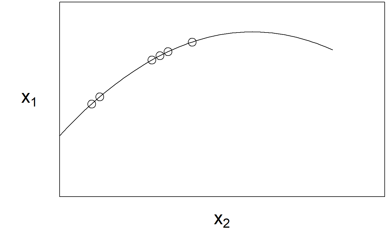
Figure 5.5: The relationship between \(x_1\) and \(x_2\) is nonlinear. However, over the region sampled, the variables have close to a linear relationship.

What can we do in the presence of collinearity? One option is to center each variable, by subtracting its average and dividing by its standard deviation. For example, create a new variable \(x_{ij}^{\ast} = (x_{ij} - \bar{x}_j) / s_{x_j}\). Occasionally, one variable appears as millions of units and another variable appears as fractions of units. Compared to the first mentioned variable, the second variable is close to a constant column of zeros (in that computers typically retain a finite number of digits). If this is true, then the second variable looks very much like a linear shift of the constant column of ones corresponding to the intercept. This is a problem because, with the least squares operations, we are implicitly squaring numbers that can make these columns appear even more similar.

This problem is simply a computational one and is easy to rectify. Simply recode the variables so that the units are of similar order of magnitude. Some data analysts automatically center all variables to avoid these problems. This is a legitimate approach because regression techniques search for linear relationships; location and scale shifts do not affect linear relationships.

Another option is to simply not explicitly account for collinearity in the analysis but to discuss some of its implications when interpreting the results of the regression analysis. This approach is probably the most commonly adopted one. It is a fact of life that, when dealing with business and economic data, collinearity does tend to exist among variables. Because the data tends to be observational in lieu of experimental in nature, there is little that the analyst can do to avoid this situation.

In the best-case situation, an auxiliary variable that provides similar information and that eases the collinearity problem is available to replace a variable. Similar to our discussion of high leverage points, a transformed version of the explanatory variable may also be a useful substitute. In some situations, such an ideal replacement is not available and we are forced to remove one or more variables. Deciding which variables to remove is a difficult choice. When deciding among variables, often the choice will be dictated by the investigator’s judgement as to which is the most relevant set of variables.

5.5.3 Collinearity and Leverage

Measures of collinearity and leverage share common characteristics and yet are designed to capture different aspects of a data set. Both are useful for data and model criticism; they are applied after a preliminary model fit with the objective of improving model specification. Further, both are calculated using only the explanatory variables; values of the responses do not enter into either calculation.

Our measure of collinearity, the variance inflation factor, is designed to help with model criticism. It is a measure calculated for each explanatory variable, designed to explain the relationship with other explanatory variables.

The leverage statistic is designed to help us with data criticism. It is a measure calculated for each observation to help us explain how unusual an observation is with respect to other observations.

Collinearity may be masked, or induced, by high leverage points, as pointed out by Mason and Gunst (1985) and Hadi (1988). Figures 5.6 and 5.7 provide illustrations of each case. These simple examples underscore an important point: data criticism and model criticism are not separate exercises.

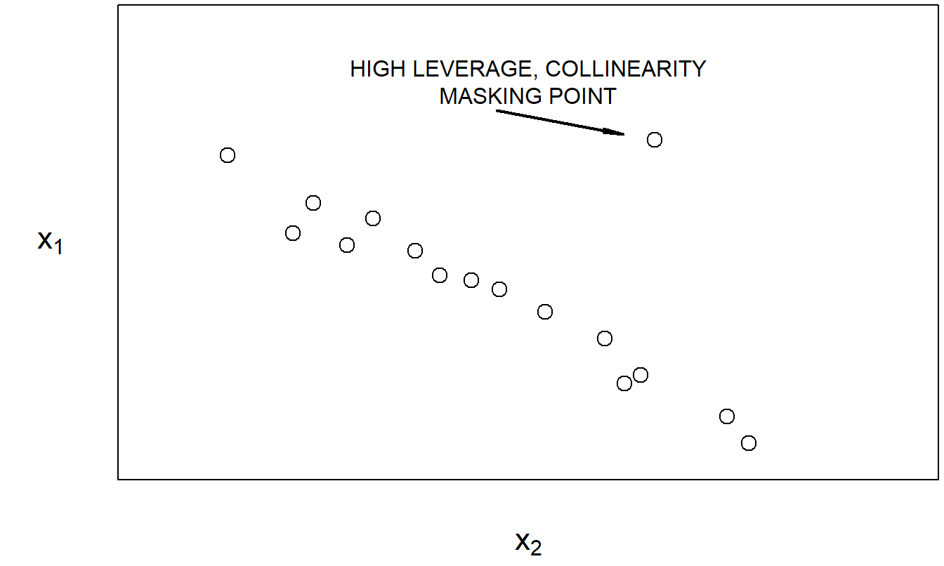
Figure 5.6: With the exception of the marked point, \(x_1\) and \(x_2\) are highly linearly related.

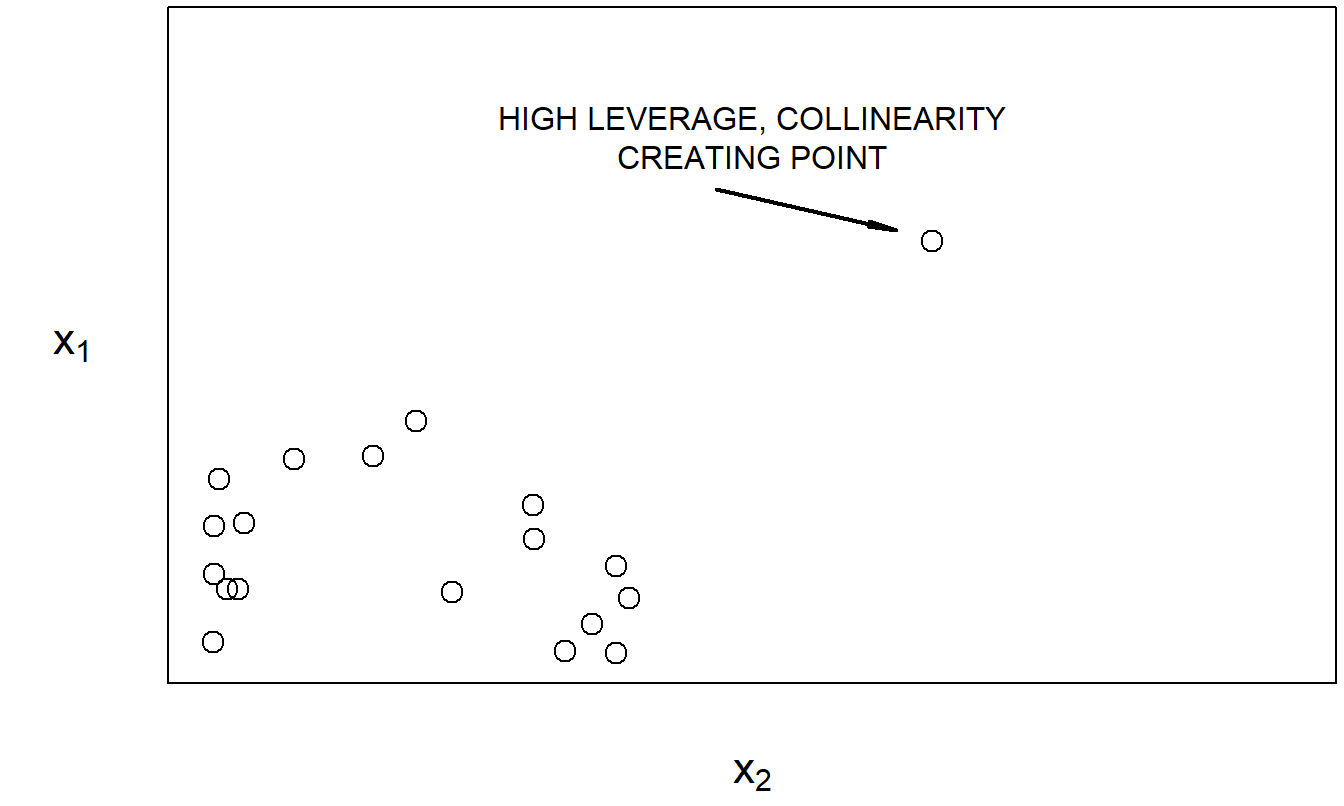
Figure 5.7: The highly linear relationship between \(x_1\) and \(x_2\) is primarily due to the marked point.

The examples in Figures 5.6 and 5.7 also help us to see one way in which high leverage points may affect standard errors of regression coefficients. Recall, in Section 5.4.1, we saw that high leverage points may affect the model fitted values. In Figures 5.6 and 5.7, we see that high leverage points affect collinearity. Thus, from equation (5.5), we have that high leverage points can also affect our standard errors of regression coefficients.

5.5.4 Suppressor Variables

As we have seen, severe collinearity can seriously inflate standard errors of regression coefficients. Because we rely on these standard errors for judging the usefulness of explanatory variables, our model selection procedures and inferences may be deficient in the presence of severe collinearity. Despite these drawbacks, mild collinearity in a data set should not be viewed as a deficiency of the data set; it is simply an attribute of the available explanatory variables.

Even if one explanatory variable is nearly a linear combination of the others, that does not necessarily mean that the information that it provides is redundant. To illustrate, we now consider a suppressor variable, an explanatory variable that increases the importance of other explanatory variables when included in the model.

Example: Suppressor Variable. Figure 5.8 shows a scatterplot matrix of a hypothetical data set of fifty observations. This data set contains a response and two explanatory variables. Table 5.8 provides the corresponding matrix of correlation coefficients. Here, we see that the two explanatory variables are highly correlated. Now recall, for regression with one explanatory variable, that the correlation coefficient squared is the coefficient of determination. Thus, using Table 5.8, for a regression of \(y\) on \(x_1\), the coefficient of determination is \((0.188)^2 = 3.5\%\). Similarly, for a regression of \(y\) on \(x_2\), the coefficient of determination is \((-0.022)^2 = 0.04\%\). However, for a regression of \(y\) on \(x_1\) and \(x_2\), the coefficient of determination turns out to be a surprisingly high \(80.7\%\). The interpretation is that individually, both \(x_1\) and \(x_2\) have little impact on \(y\). However, when taken jointly, the two explanatory variables have a significant effect on \(y\). Although Table 5.8 shows that \(x_1\) and \(x_2\) are strongly linearly related, this relationship does not mean that \(x_1\) and \(x_2\) provide the same information. In fact, in this example the two variables complement one another.

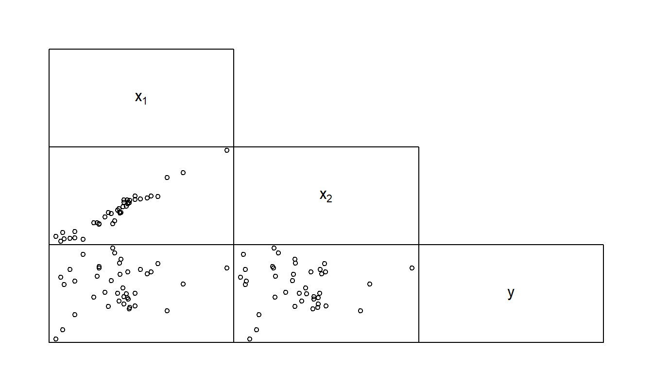
Figure 5.8: Scatterplot matrix of a response and two explanatory variables for the suppressor variable example

Table 5.8: Correlation Matrix for the Suppressor Example

	\(x_1\)	\(x_2\)
\(x_2\)	0.972
\(y\)	0.188	-0.022

5.5.5 Orthogonal Variables

Another way to understand the impact of collinearity is to study the case when there are no relationships among sets of explanatory variables. Mathematically, two matrices \(\mathbf{X}_1\) and \(\mathbf{X}_2\) are said to be orthogonal if \(\mathbf{X}_1^{\prime} \mathbf{X}_2 = \mathbf{0}\). Intuitively, because we generally work with centered variables (with zero averages), this means that each column of \(\mathbf{X}_1\) is uncorrelated with each column of \(\mathbf{X}_2\). Although unlikely to occur with observational data in the social sciences, when designing experimental treatments or constructing high degree polynomials, applications of orthogonal variables are regularly used (see for example, Hocking, 2003). For our purposes, we will work with orthogonal variables simply to understand the logical consequences of a total lack of collinearity.

Suppose that \(\mathbf{x}_2\) is an explanatory variable that is orthogonal to \(\mathbf{X}_1\), where \(\mathbf{X}_1\) is a matrix of explanatory variables that includes the intercept. Then, it is straightforward to check that the addition of \(\mathbf{x}_2\) to the regression equation does not change the fit for coefficients corresponding to \(\mathbf{X}_1\). That is, without \(\mathbf{x}_2\), the coefficients corresponding to \(\mathbf{X}_1\) would be calculated as \(\mathbf{b}_1 = \left(\mathbf{X}_1^{\prime} \mathbf{X}_1 \right)^{-1} \mathbf{X}_1^{\prime} \mathbf{y}\). Using the orthogonal \(\mathbf{x}_2\) as part of the least squares calculation would not change the result for \(\mathbf{b}_1\) (see the recursive least squares calculation in Section 4.7.2).

Further, the variance inflation factor for \(\mathbf{x}_2\) is 1, indicating that the standard error is unaffected by the other explanatory variables. In the same vein, the reduction in the error sum of squares by adding the orthogonal variable \(\mathbf{x}_2\) is due only to that variable, and not its interaction with other variables in \(\mathbf{X}_1\).

Orthogonal variables can be created for observational social science data (as well as other collinear data) using the method of principal components. With this method, one uses a linear transformation of the matrix of explanatory variables of the form, \(\mathbf{X}^{\ast} = \mathbf{X} \mathbf{P}\), so that the resulting matrix \(\mathbf{X}^{\ast}\) is composed of orthogonal columns. The transformed regression function is \(\mathrm{E~}\mathbf{y} = \mathbf{X} \boldsymbol \beta = \mathbf{X} \mathbf{P} \mathbf{P}^{-1} \boldsymbol \beta = \mathbf{X}^{\ast} \boldsymbol \beta^{\ast}\), where \(\boldsymbol \beta^{\ast} = \mathbf{P}^{-1} \boldsymbol \beta\) is the set of new regression coefficients. Estimation proceeds as before, with the orthogonal set of explanatory variables. By choosing the matrix \(\mathbf{P}\) appropriately, each column of \(\mathbf{X}^{\ast}\) has an identifiable contribution. Thus, we can readily use variable selection techniques to identify the “principal components” portions of \(\mathbf{X}^{\ast}\) to use in the regression equation. Principal components regression is a widely used method in some application areas, such as psychology. It can easily address highly collinear data in a disciplined manner. The main drawback of this technique is that the resulting parameter estimates are difficult to interpret.

Video: Section Summary

5.6 Selection Criteria

5.6.1 Goodness of Fit

How well does the model fit the data? Criteria that measure the proximity of the fitted model and realized data are known as goodness of fit statistics. Specifically, we interpret the fitted value \(\hat{y}_i\) to be the best model approximation of the \(i\)th observation and compare it to the actual value \(y_i\). In linear regression, we examine the difference through the residual \(e_i = y_i - \hat{y}_i\); small residuals imply a good model fit. We have quantified this through the size of the typical error \((s)\), including the coefficient of determination \((R^2)\) and an adjusted version \((R_{a}^2)\).

For nonlinear models, we will need additional measures, and it is helpful to introduce these measures in this simpler linear case. One such measure is Akaike’s Information Criterion that will be defined in terms of likelihood fits in Section 11.9.4. For linear regression, it reduces to

\[\begin{equation} AIC = n \ln (s^2) + n \ln (2 \pi) + n + 3 + k. \tag{5.6} \end{equation}\]

For model comparison, the smaller the \(AIC\), the better is the fit. Comparing models with the same number of variables (\(k\)) means that selecting a model with small values of \(AIC\) leads to the same choice as selecting a model with small values of the residual standard deviation \(s\). Further, a small number of parameters means a small value of \(AIC\), other things being equal. The idea is that this measure balances the fit (\(n \ln (s^2)\)) with a penalty for complexity (the number of parameters, \(k+2\)). Statistical packages often omit constants such as \(n \ln (2 \pi)\) and \(n+3\) when reporting \(AIC\) because they do not matter when comparing models.

Section 11.9.4 will introduce another measure, the Bayes Information Criterion (\(BIC\)), that gives a smaller weight to the penalty for complexity. A third goodness of fit measure that is used in linear regression models is the \(C_p\) statistic. To define this statistic, assume that we have available \(k\) explanatory variables \(x_1, ..., x_{k}\) and run a regression to get \(s_{full}^2\) as the mean square error. Now, suppose that we are considering using only \(p-1\) explanatory variables so that there are \(p\) regression coefficients. With these \(p-1\) explanatory variables, we run a regression to get the error sum of squares \((Error~SS)_p\). Thus, we are in the position to define

\[ C_{p} = \frac{(Error~SS)_p}{s_{full}^2} - n + 2p. \]

As a selection criterion, we choose the model with a “small” \(C_{p}\) coefficient, where small is taken to be relative to \(p\). In general, models with smaller values of \(C_{p}\) are more desirable.

Like the \(AIC\) and \(BIC\) statistics, the \(C_{p}\) statistic strikes a balance between the model fit and complexity. That is, each statistic summarizes the trade-off between model fit and complexity, although with different weights. For most data sets, they recommend the same model and so an analyst can report any or all three statistics. However, for some applications, they lead to different recommended models. In this case, the analyst needs to rely more heavily on non-data driven criteria for model selection (which are always important in any regression application).

5.6.2 Model Validation

Model validation is the process of confirming that our proposed model is appropriate, especially in light of the purposes of the investigation. Recall the iterative model formulation selection process described in Section 5.1. An important criticism of this iterative process is that it is guilty of data-snooping, that is, fitting a great number of models to a single set of data. As we saw in Section 5.2 on data-snooping in stepwise regression, by looking at a large number of models we may overfit the data and understate the natural variation in our representation.

We can respond to this criticism by using a technique called out-of-sample validation. The ideal situation is to have available two sets of data, one for model development and one for model validation. We initially develop one, or several, models on a first data set. The models developed from the first set of data are called our candidate models. Then, the relative performance of the candidate models could be measured on a second set of data. In this way, the data used to validate the model is unaffected by the procedures used to formulate the model.

Unfortunately, rarely will two sets of data be available to the investigator. However, we can implement the validation process by splitting the data set into two subsamples. We call these the model development and validation subsamples, respectively. They are also known as training and testing samples, respectively. To see how the process works in the linear regression context, consider the following procedure.

Out-of-Sample Validation Procedure

1. Begin with a sample size of \(n\) and divide it into two subsamples, called the model development and validation subsamples. Let \(n_1\) and \(n_2\) denote the size of each subsample. In cross-sectional regression, do this split using a random sampling mechanism. Use the notation \(i=1,...,n_1\) to represent observations from the model development subsample and \(i=n_1+1,...,n_1+n_2=n\) for the observations from the validation subsample. Figure 5.9 illustrates this procedure.
2. Using the model development subsample, fit a candidate model to the data set \(i=1,...,n_1\).
3. Using the model created in Step (ii) and the explanatory variables from the validation subsample, “predict” the dependent variables in the validation subsample, \(\hat{y}_i\), where \(i=n_1+1,...,n_1+n_2\). (To get these predictions, you may need to transform the dependent variables back to the original scale.)
4. Assess the proximity of the predictions to the held-out data. One measure is the sum of squared prediction errors \[\begin{equation} SSPE = \sum_{i=n_1+1}^{n_1+n_2} (y_i - \hat{y}_i)^2 . \tag{5.7} \end{equation}\] Repeat Steps (ii) through (iv) for each candidate model. Choose the model with the smallest SSPE.

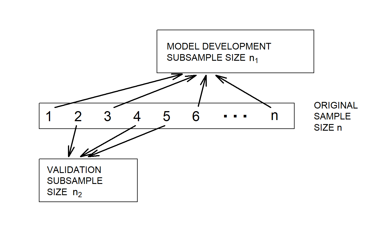
Figure 5.9: For model validation, a data set of size \(n\) is randomly split into two subsamples

There are a number of criticisms of the SSPE. First, it is clear that it takes a considerable amount of time and effort to calculate this statistic for each of several candidate models. However, as with many statistical techniques, this is merely a matter of having specialized statistical software available to perform the steps described above. Second, because the statistic itself is based on a random subset of the sample, its value will vary from analyst to analyst. This objection could be overcome by using the first \(n_1\) observations from the sample. In most applications, this is not done in case there is a lurking relationship in the order of the observations. Third, and perhaps most important, is the fact that the choice of the relative subset sizes, \(n_1\) and \(n_2\), is not clear. Various researchers recommend different proportions for the allocation. Snee (1977) suggests that data-splitting not be done unless the sample size is moderately large, specifically, \(n \geq 2(k+1) + 20\). The guidelines of Picard and Berk (1990) show that the greater the number of parameters to be estimated, the greater the proportion of observations needed for the model development subsample. As a rule of thumb, for data sets with 100 or fewer observations, use about 25-35% of the sample for out-of-sample validation. For data sets with 500 or more observations, use 50% of the sample for out-of-sample validation. Hastie, Tibshirani, and Friedman (2001) remark that a typical split is 50% for development/training, 25% for validation, and the remaining 25% for a third stage for further validation that they call testing.

Because of these criticisms, several variants of the basic out-of-sample validation process are used by analysts. Although there is no theoretically best procedure, it is widely agreed that model validation is an important part of confirming the usefulness of a model.

5.6.3 Cross-Validation

Cross-validation is the technique of model validation that splits the data into two disjoint sets. Section 5.6.2 discussed out-of-sample validation where the data was split randomly into two subsets both containing a sizeable percentage of data. Another popular method is leave-one-out cross-validation, where the validation sample consists of a single observation and the development sample is based on the remainder of the data set.

Especially for small sample sizes, an attractive leave-one-out cross-validation statistic is PRESS, the Predicted Residual Sum of Squares. To define the statistic, consider the following procedure where we suppose that a candidate model is available.

PRESS Validation Procedure

1. From the full sample, omit the \(i\)th point and use the remaining \(n-1\) observations to compute regression coefficients.
2. Use the regression coefficients computed in step one and the explanatory variables for the \(i\)th observation to compute the predicted response, \(\hat{y}_{(i)}\). This part of the procedure is similar to the calculation of the SSPE statistic with \(n_1=n-1\) and \(n_2=1\).
3. Now, repeat (i) and (ii) for \(i=1,...,n\). Summarizing, define \[\begin{equation} PRESS = \sum_{i=1}^{n} (y_i - \hat{y}_{(i)})^2 . \tag{5.8} \end{equation}\] As with SSPE, this statistic is calculated for each of several competing models. Under this criterion, we choose the model with the smallest PRESS.

Based on this definition, the statistic seems very computationally intensive in that it requires \(n\) regression fits to evaluate it. To address this, interested readers will find that Section 5.10.2 establishes

\[\begin{equation} y_i - \hat{y}_{(i)} = \frac{e_i}{1 - h_{ii}} . \tag{5.9} \end{equation}\]

Here, \(e_i\) and \(h_{ii}\) represent the \(i\)th residual and leverage from the regression fit using the complete data set. This yields

\[\begin{equation} PRESS = \sum_{i=1}^{n} \left( \frac{e_i}{1 - h_{ii}} \right)^2 , \tag{5.10} \end{equation}\]

which is a much easier computational formula. Thus, the PRESS statistic is less computationally intensive than SSPE.

Another important advantage of this statistic, when compared to SSPE, is that we do not need to make an arbitrary choice as to our relative subset sizes split. Indeed, because we are performing an “out-of-sample” validation for each observation, it can be argued that this procedure is more efficient, an especially important consideration when the sample size is small (say, less than 50 observations). A disadvantage is that because the model is re-fit for each point deleted, PRESS does not enjoy the appearance of independence between the estimation and prediction aspects, unlike SSPE.

Video: Section Summary

5.7 Heteroscedasticity

In most regression applications, the goal is to understand determinants of the regression function \(\mathrm{E~}y_i = \mathbf{x}_i^{\prime} \boldsymbol \beta = \mu_i\). Our ability to understand the mean is strongly influenced by the amount of spread from the mean that we quantify using the variance \(\mathrm{E}\left(y_i - \mu_i\right)^2\). In some applications, such as when I weigh myself on a scale, there is relatively little variability; repeated measurements yield almost the same result. In other applications, such as the time it takes me to fly to New York, repeated measurements yield substantial variability and are fraught with inherent uncertainty.

The amount of uncertainty can also vary on a case-by-case basis. We denote the case of “varying variability” with the notation \(\sigma_i^2 = \mathrm{E}\left(y_i - \mu_i\right)^2\). When the variability varies by observation, this is known as heteroscedasticity for “different scatter.” In contrast, the usual assumption of common variability (assumption E3/F3 in Section 3.2) is called homoscedasticity, meaning “same scatter.”

Our estimation strategies depend on the extent of heteroscedasticity. For datasets with only a mild amount of heteroscedasticity, one can use least squares to estimate the regression coefficients, perhaps combined with an adjustment for the standard errors (described in Section 5.7.2). This is because least squares estimators are unbiased even in the presence of heteroscedasticity (see Property 1 in Section 3.2).

However, with heteroscedastic dependent variables, the Gauss-Markov theorem no longer applies and so the least squares estimators are not guaranteed to be optimal. In cases of severe heteroscedasticity, alternative estimators are used, the most common being those based on transformations of the dependent variable, as will be described in Section 5.7.4.

5.7.1 Detecting Heteroscedasticity

To decide a strategy for handling potential heteroscedasticity, we must first assess, or detect, its presence.

To detect heteroscedasticity graphically, a good idea is to perform a preliminary regression fit of the data and plot the residuals versus the fitted values. To illustrate, Figure 5.10 is a plot of a fictitious data set with one explanatory variable where the scatter increases as the explanatory variable increases. A least squares regression was performed - residuals and fitted values were computed. Figure 5.11 is an example of a plot of residuals versus fitted values. The preliminary regression fit removes many of the major patterns in the data and leaves the eye free to concentrate on other patterns that may influence the fit. We plot residuals versus fitted values because the fitted values are an approximation of the expected value of the response and, in many situations, the variability grows with the expected response.

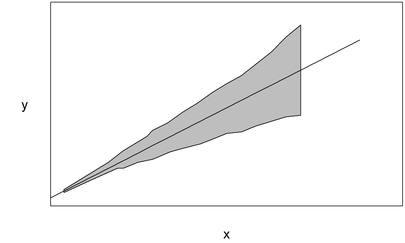
Figure 5.10: The shaded area represents the data.

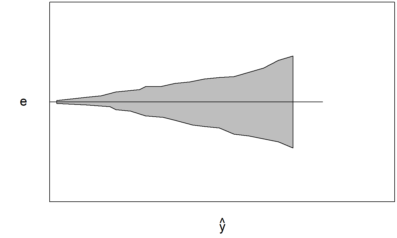
Figure 5.11: Residuals plotted versus the fitted values for the data in Figure 5.10.

More formal tests of heteroscedasticity are also available in the regression literature. To illustrate, let us consider a test due to Breusch and Pagan (1980). Specifically, this test examines the alternative hypothesis \(H_a\): \(\mathrm{Var~} y_i = \sigma^2 + \mathbf{z}_i^{\prime} \boldsymbol \gamma\), where \(\mathbf{z}_i\) is a known vector of variables and \(\boldsymbol \gamma\) is a \(p\)-dimensional vector of parameters. Thus, the null hypothesis is \(H_0:~ \boldsymbol \gamma = \mathbf{0}\) is equivalent to homoscedasticity, \(\mathrm{Var~} y_i = \sigma^2.\)

Procedure to Test for Heteroscedasticity

1. Fit a regression model and calculate the model residuals, \(e_i\).
2. Calculate squared standardized residuals, \(e_i^{\ast 2} = e_i^2 / s^2\).
3. Fit a regression model of \(e_i^{\ast 2}\) on \(\mathbf{z}_i\).
4. The test statistic is \(LM = \frac{\text{Regress~SS}_z}{2}\), where \(Regress~SS_z\) is the regression sum of squares from the model fit in step (iii).
5. Reject the null hypothesis if \(LM\) exceeds a percentile from a chi-square distribution with \(p\) degrees of freedom. The percentile is one minus the significance level of the test.

Here, we use \(LM\) to denote the test statistic because Breusch and Pagan derived it as a Lagrange multiplier statistic; see Breusch and Pagan (1980) for more details.

5.7.2 Heteroscedasticity-Consistent Standard Errors

For data sets with only mild heteroscedasticity, a sensible strategy is to employ least squares estimators of the regression coefficients and to adjust the calculation of standard errors to account for the heteroscedasticity.

From the Section 3.2 on properties, we saw that least squares regression coefficients could be written as \(\mathbf{b} = \sum_{i=1}^n \mathbf{w}_i y_i,\) where \(\mathbf{w}_i = \left( \mathbf{X}^{\prime}\mathbf{X} \right)^{-1} \mathbf{x}_i\). Thus, with \(\sigma_i^2 = \mathrm{Var~} y_i\), we have \[\begin{equation} \mathrm{Var~}\mathbf{b} = \sum_{i=1}^n \mathbf{w}_i \mathbf{w}_i^{\prime} \sigma_i^2 = \left( \mathbf{X}^{\prime}\mathbf{X} \right)^{-1} \left( \sum_{i=1}^n \sigma_i^2 \mathbf{x}_i \mathbf{x}_i^{\prime} \right) \left( \mathbf{X}^{\prime}\mathbf{X} \right)^{-1}. \tag{5.11} \end{equation}\] This quantity is known except for \(\sigma_i^2\). We can compute residuals using the least squares regression coefficients as \(e_i = y_i - \mathbf{x}_i^{\prime} \mathbf{b}\). With these, we may define the empirical, or robust, estimate of the variance-covariance matrix as \[ \widehat{\mathrm{Var~}\mathbf{b}} = \left( \mathbf{X}^{\prime}\mathbf{X} \right)^{-1} \left( \sum_{i=1}^n e_i^2 \mathbf{x}_i \mathbf{x}_i^{\prime} \right) \left( \mathbf{X}^{\prime}\mathbf{X} \right)^{-1}. \] The corresponding “heteroscedasticity-consistent” standard errors are \[\begin{equation} se_r(b_j) = \sqrt{(j+1)^{\text{st}}~ \text{diagonal element of }\widehat{\mathrm{Var~}\mathbf{b}}}. \tag{5.12} \end{equation}\] The logic behind this estimator is that each squared residual, \(e_i^2\), may be a poor estimate of \(\sigma_i^2\). However, our interest is estimating a (weighted) sum of variances in equation (5.11); estimating the sum is a much easier task than estimating any individual variance estimate.

Robust, or heteroscedasticity-consistent, standard errors are widely available in statistical software packages. Here, you will also see alternative definitions of residuals employed, as in Section 5.3.1. If your statistical package offers options, the robust estimator using studentized residuals is generally preferred.

5.7.3 Weighted Least Squares

The least squares estimators are less useful for datasets with severe heteroscedasticity. One strategy is to use a variation of least squares estimation by weighting observations. The idea is that, when minimizing the sum of squared errors using heteroscedastic data, the expected variability of some observations is smaller than others. Intuitively, it seems reasonable that the smaller the variability of the response, the more reliable that response and the greater weight that it should receive in the minimization procedure. Weighted least squares is a technique that accounts for this “varying variability.”

Specifically, we use Section 3.2.3 assumptions E1, E2, and E4, with E3 replaced by E \(\varepsilon_i = 0\) and \(\text{Var} \varepsilon_i = \sigma^2 / w_i\), so that the variability is proportional to a known weight \(w_i\). For example, if unit of analysis \(i\) represents a geographical entity such as a state, you might use the number of people in the state as a weight. Or, if \(i\) represents a firm, you might use firm assets for the weighting variable. Larger values of \(w_i\) indicate a more precise response variable through the smaller variability. In actuarial applications, weights are used to account for an exposure such as the amount of insurance premium, number of employees, size of the payroll, number of insured vehicles, and so forth (further discussion is in Chapter 18).

This model can be readily converted to the “ordinary” least squares problem by multiplying all regression variables by \(\sqrt{w_i}\). That is, if we define \(y_i^{\ast} = y_i \times \sqrt{w_i}\) and \(x_{ij}^{\ast} = x_{ij} \times \sqrt{w_i}\), then from assumption E1 we have \[ \begin{array}{ll} y_i^{\ast} & = y_i \times \sqrt{w_i} = \left( \beta_0 x_{i0} + \beta_1 x_{i1} + \ldots + \beta_k x_{ik} + \varepsilon_i \right) \sqrt{w_i} \\ &= \beta_0 x_{i0}^{\ast} + \beta_1 x_{i1}^{\ast} + \ldots + \beta_k x_{ik}^{\ast} + \varepsilon_i^{\ast} \end{array} \] where \(\varepsilon_i^{\ast} = \varepsilon_i \times \sqrt{w_i}\) has homoscedastic variance \(\sigma^2\). Thus, with the rescaled variables, all inference can proceed as before.

This work has been automated in statistical packages where the user merely specifies the weights \(w_i\) and the package does the rest. In terms of matrix algebra, this procedure can be accomplished by defining an \(n \times n\) weight matrix \(\mathbf{W} = \text{diag}(w_i)\) so that the \(i\)th diagonal element of \(\mathbf{W}\) is \(w_i\). Extending equation (3.14) for example, the weighted least squares estimates can be expressed as \[\begin{equation} \mathbf{b}_{WLS} = \left( \mathbf{X}^{\prime} \mathbf{W} \mathbf{X} \right)^{-1} \mathbf{X}^{\prime} \mathbf{W} \mathbf{y}. \tag{5.13} \end{equation}\] Additional discussions of weighted least squares estimation will be presented in Section 15.1.1.

5.7.4 Transformations

Another approach that handles severe heteroscedasticity, introduced in Section 1.3, is to transform the dependent variable, typically with a logarithmic transformation of the form \(y^{\ast} = \ln y\). As we saw in Section 1.3, transformations can serve to “shrink” spread out data and symmetrize a distribution. Through a change of scale, a transformation also changes the variability, potentially altering a heteroscedastic dataset into a homoscedastic one. This is both a strength and limitation of the transformation approach - a transformation simultaneously affects both the distribution and the heteroscedasticity.

Power transformations, such as the logarithmic transform, are most useful when the variability of the data grows with the mean. In this case, the transform will serve to “shrink” the data to a scale that appears to be homoscedastic. Conversely, because transformations are monotonic functions, they will not help with patterns of variability that are non-monotonic. Further, if your data is reasonably symmetric but heteroscedastic, a transformation will not be useful because any choice that mitigates the heteroscedasticity will skew the distribution.

When data are non-positive, it is common to add a constant to each observation so that all observations are positive prior to transformation. For example, the transform \(\ln(1+y)\) accommodates the presence of zeros. One can also multiply by a constant so that the approximate original units are retained. For example, the transform \(100 \ln(1 + y/100)\) may be applied to percentage data where negative percentages sometimes appear.

Our discussions of transformations have focused on transforming dependent variables. As noted in Section 3.5, transformations of explanatory variables are also possible. This is because the regression assumptions condition on explanatory variables (Section 3.2.3). Some analysts prefer to transform variables to approximate normality, thinking of multivariate normal distributions as a foundation for regression analysis. Others are reluctant to transform explanatory variables because of the difficulties in interpreting resulting models. The approach taken here is to use transforms that can be readily interpretable, such as those introduced in Section 3.5. Other transforms are certainly candidates to include in a selected model but they should provide substantial dividends in terms of fit or predictive power if they are difficult to communicate.

Video: Section Summary

5.8 Further Reading and References

Long and Ervin (2000) gather compelling evidence for the use of alternative heteroscedasticity-consistent estimators of standard errors that have better finite sample performance than the classic versions. The large sample properties of empirical estimators have been established by Eicker (1967), Huber (1967) and White (1980) in the linear regression case. For the linear regression case, MacKinnon and White (1985) suggest alternatives that provide superior small-sample properties. For small samples, the evidence is based on (1) the biasedness of the estimators, (2) their motivation as jackknife estimators and (3) their performance in simulation studies.

Other measures of collinearity based on matrix algebra concepts involving eigenvalues, such as condition numbers and condition indices, are used by some analysts. See Belseley, Kuh and Welsch (1980) for a solid treatment of collinearity and regression diagnostics. Hocking (2003) provides additional background reading on collinearity and principal components. See Carroll and Ruppert (1988) for further discussions of transformations in regression.

Hastie, Tibshirani and Friedman (2001) give an advanced discussion of model selection issues, focusing on predictive aspects of models in the language of machine learning.

Chapter References

• Belseley, David A., Edwin Kuh and Roy E. Welsch (1980). Regression Diagnostics: Identifying Influential Data and Sources of Collinearity. Wiley, New York.
• Bendel, R. B. and Afifi, A. A. (1977). Comparison of stopping rules in forward “stepwise” regression. Journal of the American Statistical Association 72, 46-53.
• Box, George E. P. (1980). Sampling and Bayes inference in scientific modeling and robustness (with discussion). Journal of the Royal Statistical Society, Series A, 143, 383-430.
• Breusch, T. S. and A. R. Pagan (1980). The Lagrange multiplier test and its applications to model specification in econometrics. Review of Economic Studies, 47, 239-53.
• Carroll, Raymond J. and David Ruppert (1988). Transformation and Weighting in Regression, Chapman-Hall.
• Eicker, F. (1967). Limit theorems for regressions with unequal and dependent errors. Proceedings of the Fifth Berkeley Symposium on Mathematical Statistics and Probability 1, LeCam, L. M. and J. Neyman, editors, University of California Press, pp, 59-82.
• Hadi, A. S. (1988). Diagnosing collinearity-influential observations. Computational Statistics and Data Analysis 7, 143-159.
• Hastie, Trevor, Robert Tibshirani and Jerome Friedman (2001). The Elements of Statistical Learning: Data Mining, Inference and Prediction. Springer-Verlag, New York.
• Hocking, Ronald R. (2003). Methods and Applications of Linear Models: Regression and the Analysis of Variance. Wiley, New York.
• Huber, P. J. (1967). The behaviour of maximum likelihood estimators under non-standard conditions. Proceedings of the Fifth Berkeley Symposium on Mathematical Statistics and Probability 1, LeCam, L. M. and Neyman, J. editors, University of California Press, pp, 221-33.
• Long, J.S. and L.H. Ervin (2000). Using heteroscedasticity consistent standard errors in the linear regression model. American Statistician 54, 217-224.
• MacKinnon, J.G. and H. White (1985). Some heteroskedasticity consistent covariance matrix estimators with improved finite sample properties. Journal of Econometrics 29, 53-57.
• Mason, R. L. and Gunst, R. F. (1985). Outlier-induced collinearities. Technometrics 27, 401-407.
• Picard, R. R. and Berk, K. N. (1990). Data splitting. The American Statistician 44, 140-147.
• Rencher, A. C. and Pun, F. C. (1980). Inflation of \(R^2\) in best subset regression. Technometrics 22, 49-53.
• Snee, R. D. (1977). Validation of regression models. Methods and examples. Technometrics 19, 415-428.

5.9 Exercises

5.1. You are doing regression with one explanatory variable and so consider the basic linear regression model \(y_i = \beta_0 + \beta_1 x_i + \varepsilon_i\).

1. Show that the \(i\)th leverage can be simplified to \[ h_{ii} = \frac{1}{n} + \frac{(x_i - \overline{x})^2}{(n-1) s_x^2}. \]
2. Show that \(\overline{h} = 2 / n\).
3. Suppose that \(h_{ii} = 6/n\). How many standard deviations is \(x_i\) away (either above or below) from the mean?

5.2. Consider the output of a regression using one explanatory variable on \(n=3\) observations. The residuals and leverages are: \[ \small{ \begin{array}{l|ccc} \hline i & 1 & 2 & 3 \\ \hline \text{Residuals } e_i & 3.181 & -6.362 & 3.181 \\ \text{Leverages } h_{ii} & 0.8333 & 0.3333 & 0.8333 \\ \hline \end{array} } \]

Compute the \(PRESS\) statistic.

5.3. National Life Expectancies. We continue the analysis begun in Exercises 1.7, 2.22, 3.6 and 4.7. The focus of this exercise is variable selection.

1. Begin with the data from \(n=185\) countries throughout the world that have valid (non-missing) life expectancies. Plot the life expectancy versus the gross domestic product and private expenditures on health. From these plots, describe why it is desirable to use logarithmic transforms, lnGDP and lnHEALTH, respectively. Also plot life expectancy versus lnGDP and lnHEALTH to confirm your intuition.

2. Use a stepwise regression algorithm to help you select a model. Do not consider the variables RESEARCHERS, SMOKING, and FEMALEBOSS as these have many missing values. For the remaining variables, use only the observations without any missing values. Do this twice, with and without the categorical variable EGION.

3. Return to the full data set of \(n=185\) countries and run a regression model using FERTILITY, PUBLICEDUCATION, and lnHEALTH as explanatory variables.

   c(i). Provide histograms of standardized residuals and leverages.
   c(ii). Identify the standardized residual and leverage associated with Lesotho, formerly Basutoland, a kingdom surrounded by South Africa. Is this observation an outlier, high leverage point, or both?
   c(iii). Re-run the regression without Lesotho. Cite any differences in the statistical coefficients between this model and the one in part c(i).

5.4. Term Life Insurance. We continue our study of Term Life Insurance Demand from Chapters 3 and 4. Specifically, we examine the 2004 Survey of Consumer Finances (SCF), a nationally representative sample that contains extensive information on assets, liabilities, income, and demographic characteristics of those sampled (potential U.S. customers). We study a random sample of 500 families with positive incomes. From the sample of 500, we initially consider a subsample of \(n=275\) families that purchased term life insurance.

Consider a linear regression of LNINCOME, EDUCATION, NUMHH, MARSTAT, AGE, and GENDER on LNFACE}.

1. Collinearity. Not all of the variables turned out to be statistically significant. To investigate one possible explanation, calculate variance inflation factors.

   a(i). Briefly explain the idea of collinearity and a variance inflation factor.
   a(ii). What constitutes a large variance inflation factor?
   a(iii). If a large variance inflation factor is detected, what possible courses of action do we have to address this aspect of the data?
   a(iv). Supplement the variance inflation factor statistics with a table of correlations of explanatory variables. Based on these statistics, is collinearity an issue with this fitted model? Why or why not?

2. Unusual Points. Sometimes a poor model fit can be due to unusual points.

   b(i). Define the idea of leverage for an observation.
   b(ii). For this fitted model, give standard rules of thumb for identifying points with unusual leverage. Identify any unusual points.
   b(iii). An analyst is concerned with leverage values for this fitted model and suggests using FACE as the dependent variable instead of LNFACE. Describe how leverage values would change using this alternative dependent variable.

3. Residual Analysis. We can learn how to improve model fits from analyses of residuals.

   c(i). Provide a plot of residuals versus fitted values. What do we hope to learn from this type of plot? Does this plot display any model inadequacies?
   c(ii). Provide a \(qq\) plot of residuals. What do we hope to learn from this type of plot? Does this plot display any model inadequacies?
   c(iii). Provide a plot of residuals versus leverages. What do we hope to learn from this type of plot? Does this plot display any model inadequacies?

4. Stepwise Regression. Run a stepwise regression algorithm. Suppose that this algorithm suggests a model using LNINCOME}, EDUCATION, NUMHH, and GENDER as explanatory variables to predict the dependent variable LNFACE.

   d(i). What is the purpose of stepwise regression?
   d(ii). Describe two important drawbacks of stepwise regression algorithms.

5.10 Technical Supplements for Chapter 5

5.10.1 Projection Matrix

Hat Matrix. We define the hat matrix to be \(\mathbf{H} = \mathbf{X(X}^{\prime}\mathbf{X)}^{-1} \mathbf{X}^{\prime}\), so that \(\mathbf{\hat{y}} = \mathbf{X b} = \mathbf{Hy}\). From this, the matrix \(\mathbf{H}\) is said to project the vector of responses \(\mathbf{y}\) onto the vector of fitted values \(\mathbf{\hat{y}}\).

Because \(\mathbf{H}^{\prime} = \mathbf{H}\), the hat matrix is symmetric. Further, it is also an idempotent matrix due to the property that \(\mathbf{HH} = \mathbf{H}\). To see this, we have that \[ \begin{array}{ll} \mathbf{HH} &= \mathbf{(X(\mathbf{X}^{\prime}X)}^{-1}\mathbf{X}^{\prime}\mathbf{)(X(\mathbf{X}^{\prime}X)}^{-1}\mathbf{X}^{\prime}\mathbf{)} \\ &= \mathbf{X(\mathbf{X}^{\prime}X)}^{-1}\mathbf{(\mathbf{X}^{\prime}X)(\mathbf{X}^{\prime}X)}^{-1}\mathbf{X}^{\prime} = \mathbf{X(\mathbf{X}^{\prime}X)}^{-1}\mathbf{X}^{\prime} = \mathbf{H}. \end{array} \] Similarly, it is easy to check that \(\mathbf{I-H}\) is idempotent. Because \(\mathbf{H}\) is idempotent, from some results in matrix algebra, it is straightforward to show that \[ \sum_{i=1}^{n} h_{ii} = k + 1. \] As discussed in Section 5.4.1, we use our bounds and the average leverage, \(\bar{h} = (k + 1)/n\), to help identify observations with unusually high leverage.

Variance of Residuals. Using the model equation \(\mathbf{y} = \mathbf{X} \boldsymbol{\beta} + \boldsymbol{\varepsilon}\), we can express the vector of residuals as \[\begin{equation} \mathbf{e} = \mathbf{y} - \mathbf{\hat{y}} = \mathbf{y - Hy} = \mathbf{(I-H)(X \boldsymbol{\beta} + \boldsymbol{\varepsilon})} = \mathbf{(I-H) \boldsymbol{\varepsilon}}. \tag{5.14} \end{equation}\] The last equality is due to the fact that \(\mathbf{(I-H)X} = \mathbf{X - HX} = \mathbf{X - X} = \mathbf{0}\). Using \(\text{Var}~ \boldsymbol{\varepsilon} = \sigma^2 \mathbf{I}\), we have \[ \begin{array}{ll} \text{Var } \mathbf{e} &= \text{Var }\left[ \mathbf{(I-H)\boldsymbol{\varepsilon}} \right] = \mathbf{(I-H)} \text{Var } \boldsymbol{\varepsilon} \mathbf{(I-H)} \\ &= \sigma^2 \mathbf{(I-H)} \mathbf{I} \mathbf{(I-H)} = \sigma^2 \mathbf{(I-H)}. \end{array} \] The last equality comes from the fact that \(\mathbf{I-H}\) is idempotent. Thus, we have that \[\begin{equation} \text{Var } e_i = \sigma^2 (1 - h_{ii}) \text{ and Cov } (e_i, e_j) = -\sigma^2 h_{ij}. \tag{5.15} \end{equation}\] Thus, although the true errors \(\boldsymbol{\varepsilon}\) are uncorrelated, there is a small negative correlation among residuals \(\mathbf{e}\).

Dominance of the Error in the Residual. Examining the \(i\)th row of equation (5.14), we have that the \(i\)th residual \[\begin{equation} e_i = \varepsilon_i - \sum_{j=1}^{n} h_{ij} \varepsilon_j \tag{5.16} \end{equation}\] can be expressed as a linear combination of independent errors. The relation \(\mathbf{H} = \mathbf{HH}\) yields \[\begin{equation} h_{ii} = \sum_{j=1}^{n} h_{ij}^2. \tag{5.17} \end{equation}\] Because \(h_{ii}\) is, on average, \((k + 1)/n\), this indicates that each \(h_{ij}\) is small relative to 1. Thus, when interpreting equation (5.16), we say that most of the information in \(e_i\) is due to \(\varepsilon_i\).

Correlations with Residuals. First define \(\mathbf{x}^j = (x_{1j}, x_{2j}, \dots, x_{nj})^{\prime}\) to be the column representing the \(j\)th variable. With this notation, we can partition the matrix of explanatory variables as \(\mathbf{X} = \left( \mathbf{x}^{0}, \mathbf{x}^{1}, \dots, \mathbf{x}^{k} \right)\). Now, examining the \(j\)th column of the relation \(\mathbf{(I-H)X} = \mathbf{0}\), we have \(\mathbf{(I-H)x}^{j} = \mathbf{0}\). With \(\mathbf{e} = \mathbf{(I-H) \boldsymbol{\varepsilon}}\), this yields \[ \mathbf{e}^{\prime} \mathbf{x}^{j} = \boldsymbol{\varepsilon}^{\prime} \mathbf{(I-H)x}^{j} = 0, \] for \(j = 0, 1, \ldots, k.\) This result has several implications. If the intercept is in the model, then \(\mathbf{x}^{0} = (1, 1, \ldots, 1)^{\prime}\) is a vector of ones. Here, \(\mathbf{e}^{\prime} \mathbf{x}^{0} = 0\) means that \(\sum_{i=1}^{n} e_i = 0\) or, the average residual is zero. Further, because \(\mathbf{e}^{\prime} \mathbf{x}^{j} = 0\), it is easy to check that the sample correlation between \(\mathbf{e}\) and \(\mathbf{x}^{j}\) is zero. Along the same line, we also have that \(\mathbf{e}^{\prime} \mathbf{\hat{y}} = \mathbf{e}^{\prime} \mathbf{(I-H)Xb} = \mathbf{0}\). Thus, using the same argument as above, the sample correlation between \(\mathbf{e}\) and \(\mathbf{\hat{y}}\) is zero.

Multiple Correlation Coefficient. For an example of a non-zero correlation, consider \(r(\mathbf{y, \hat{y}})\), the sample correlation between \(\mathbf{y}\) and \(\mathbf{\hat{y}}\). Because \(\mathbf{(I-H)x}^{0} = \mathbf{0}\), we have \(\mathbf{x}^{0} = \mathbf{Hx}^{0}\) and thus, \(\mathbf{\hat{y}}^{\prime} \mathbf{x}^{0} = \mathbf{y}^{\prime} \mathbf{Hx}^{0} = \mathbf{y^{\prime} x}^{0}\). Assuming \(\mathbf{x}^{0} = (1, 1, \ldots, 1)^{\prime}\), this means that \(\sum_{i=1}^{n} \hat{y}_i = \sum_{i=1}^{n} y_i\), so that the average fitted value is \(\bar{y}\).

\[ r(\mathbf{y, \hat{y}}) = \frac{\sum_{i=1}^{n} (y_i - \bar{y})(\hat{y}_i - \bar{y})}{(n-1) s_y s_{\hat{y}}}. \]

Recall that \((n-1) s_y^2 = \sum_{i=1}^{n} (y_i - \bar{y})^2 = Total ~SS\) and \((n-1) s_{\hat{y}}^2 = \sum_{i=1}^{n} (\hat{y}_i - \bar{y})^2 = Regress ~SS\). Further, with \(\mathbf{x}^0 = (1, 1, \ldots, 1)^{\prime}\), \[ \begin{array}{ll} \sum_{i=1}^{n} (y_i - \bar{y})(\hat{y}_i - \bar{y}) &= (\mathbf{y} - \bar{y} \mathbf{x}^0)^{\prime} (\mathbf{\hat{y}} - \bar{y} \mathbf{x}^0) = \mathbf{y}^{\prime} \mathbf{\hat{y}} - \bar{y}^2 \mathbf{x}^{0 \prime} \mathbf{x}^0 \\ &= \mathbf{y}^{\prime} \mathbf{Xb} - n \bar{y}^2 = Regress ~SS. \end{array} \]

This yields \[\begin{equation} r(\mathbf{y, \hat{y}}) = \frac{Regress ~SS}{\sqrt{\left( Total ~SS \right) \left( Regress ~SS \right)}} = \sqrt{\frac{Regress ~SS}{Total ~SS}} = \sqrt{R^2}. \tag{5.18} \end{equation}\] That is, the coefficient of determination can be interpreted as the square root of the correlation between the observed and fitted responses.

5.10.2 Leave One Out Statistics

Notation. To test the sensitivity of regression quantities, there are a number of statistics of interest that are based on the notion of “leaving out,” or omitting, an observation. To this end, the subscript notation \((i)\) means to leave out the \(i\)th observation. For example, omitting the row of explanatory variables \(\mathbf{x}_i^{\prime} = (x_{i0}, x_{i1}, \dots, x_{ik})\) from \(\mathbf{X}\) yields \(\mathbf{X}_{(i)}\), a \((n-1) \times (k+1)\) matrix of explanatory variables. Similarly, \(\mathbf{y}_{(i)}\) is a \((n-1) \times 1\) vector, based on removing the \(i\)th row from \(\mathbf{y}\).

Basic Matrix Result. Suppose that \(\mathbf{A}\) is an invertible, \(p \times p\) matrix and \(\mathbf{z}\) is a \(p \times 1\) vector. The following result from matrix algebra provides an important tool for understanding leave one out statistics in linear regression analysis. \[\begin{equation} \left( \mathbf{A - zz}^{\prime} \right)^{-1} = \mathbf{A}^{-1} + \frac{\mathbf{A}^{-1} \mathbf{zz}^{\prime} \mathbf{A}^{-1}}{1 - \mathbf{z}^{\prime} \mathbf{A}^{-1} \mathbf{z}}. \tag{5.19} \end{equation}\] To check this result, simply multiply \(\mathbf{A - zz}^{\prime}\) by the right hand side of the equation to get \(\mathbf{I}\), the identity matrix.

Vector of Regression Coefficients. Omitting the \(i\)th observation, our new vector of regression coefficients is \(\mathbf{b}_{(i)} = \left( \mathbf{X}_{(i)}^{\prime} \mathbf{X}_{(i)} \right)^{-1} \mathbf{X}_{(i)}^{\prime} \mathbf{y}_{(i)}.\) An alternative expression for \(\mathbf{b}_{(i)}\) that is simpler to compute turns out to be \[\begin{equation} \mathbf{b}_{(i)} = \mathbf{b} - \frac{\left( \mathbf{X}^{\prime} \mathbf{X} \right)^{-1} \mathbf{x}_i e_i}{1 - h_{ii}}.S \tag{5.20} \end{equation}\] To verify this, first use the matrix inversion result with \(\mathbf{A} = \mathbf{X}^{\prime} \mathbf{X}\) and \(\mathbf{z} = \mathbf{x}_i\) to get \[ \left( \mathbf{X}_{(i)}^{\prime} \mathbf{X}_{(i)} \right)^{-1} = (\mathbf{X}^{\prime} \mathbf{X} - \mathbf{x}_i \mathbf{x}_i^{\prime})^{-1} = (\mathbf{X}^{\prime} \mathbf{X})^{-1} + \frac{\left( \mathbf{X}^{\prime} \mathbf{X} \right)^{-1} \mathbf{x}_i \mathbf{x}_i^{\prime} \left( \mathbf{X}^{\prime} \mathbf{X} \right)^{-1}}{1 - h_{ii}}, \] where, from the leverage result, we have \(h_{ii} = \mathbf{x}_i^{\prime} (\mathbf{X}^{\prime} \mathbf{X})^{-1} \mathbf{x}_i\). Multiplying each side by \[ \mathbf{X}_{(i)}^{\prime} \mathbf{y}_{(i)} = \mathbf{X}^{\prime} \mathbf{y} - \mathbf{x}_i y_i \] yields \[ \begin{array}{ll} \mathbf{b}_{(i)} &= \left( \mathbf{X}_{(i)}^{\prime} \mathbf{X}_{(i)} \right)^{-1} \mathbf{X}_{(i)}^{\prime} \mathbf{y}_{(i)} \\ &= \left( (\mathbf{X}^{\prime} \mathbf{X})^{-1} + \frac{\left( \mathbf{X}^{\prime} \mathbf{X} \right)^{-1} \mathbf{x}_i \mathbf{x}_i^{\prime} \left( \mathbf{X}^{\prime} \mathbf{X} \right)^{-1}}{1 - h_{ii}} \right) \left( \mathbf{X}^{\prime} \mathbf{y} - \mathbf{x}_i y_i \right) \\ &= \mathbf{b} - \left( \mathbf{X}^{\prime} \mathbf{X} \right)^{-1} \mathbf{x}_i y_i + \frac{\left( \mathbf{X}^{\prime} \mathbf{X} \right)^{-1} \mathbf{x}_i \mathbf{x}_i^{\prime} \mathbf{b} - \left( \mathbf{X}^{\prime} \mathbf{X} \right)^{-1} \mathbf{x}_i \mathbf{x}_i^{\prime} \left( \mathbf{X}^{\prime} \mathbf{X} \right)^{-1} \mathbf{x}_i y_i}{1 - h_{ii}} \\ &= \mathbf{b} - \frac{\left( 1 - h_{ii} \right) \left( \mathbf{X}^{\prime} \mathbf{X} \right)^{-1} \mathbf{x}_i y_i - \left( \mathbf{X}^{\prime} \mathbf{X} \right)^{-1} \mathbf{x}_i \mathbf{x}_i^{\prime} \mathbf{b} - \left( \mathbf{X}^{\prime} \mathbf{X} \right)^{-1} \mathbf{x}_i h_{ii} y_i}{1 - h_{ii}} \\ &= \mathbf{b} - \frac{\left( \mathbf{X}^{\prime} \mathbf{X} \right)^{-1} \mathbf{x}_i y_i - \left( \mathbf{X}^{\prime} \mathbf{X} \right)^{-1} \mathbf{x}_i \mathbf{x}_i^{\prime} \mathbf{b}}{1 - h_{ii}} \\ &= \mathbf{b} - \frac{\left( \mathbf{X}^{\prime} \mathbf{X} \right)^{-1} \mathbf{x}_i e_i}{1 - h_{ii}}. \end{array} \] This establishes the result.

Cook’s Distance. To measure the effect, or influence, of omitting the \(i\)th observation, Cook examined the difference between fitted values with and without the observation. We define Cook’s Distance to be \[ D_i = \frac{\left( \mathbf{\hat{y} - \hat{y}}_{(i)} \right)^{\prime} \left( \mathbf{\hat{y} - \hat{y}}_{(i)} \right)}{(k+1) s^2} \] where \(\mathbf{\hat{y}}_{(i)} = \mathbf{Xb}_{(i)}\) is the vector of fitted values calculated omitting the \(i\)th point. Using equation (5.20) and \(\mathbf{\hat{y}} = \mathbf{Xb}\), an alternative expression for Cook’s Distance is \[ \begin{array}{ll} D_i &= \frac{\left( \mathbf{b - b}_{(i)} \right)^{\prime} \left( \mathbf{X}^{\prime} \mathbf{X} \right) \left( \mathbf{b - b}_{(i)} \right)}{(k+1) s^2} \\ &= \frac{e_i^2}{(1 - h_{ii})^2} \frac{\mathbf{x}_i^{\prime} \left( \mathbf{X}^{\prime} \mathbf{X} \right)^{-1} \left( \mathbf{X}^{\prime} \mathbf{X} \right) \left( \mathbf{X}^{\prime} \mathbf{X} \right)^{-1} \mathbf{x}_i}{(k+1) s^2} \\ & = \frac{e_i^2}{(1 - h_{ii})^2} \frac{h_{ii}}{(k+1) s^2} \\ &= \left( \frac{e_i}{s \sqrt{1 - h_{ii}}} \right)^2 \frac{h_{ii}}{(k+1) (1 - h_{ii})}. \end{array} \] This result is not only useful computationally, it also serves to decompose the statistic into the part due to the standardized residual, \((e_i/(s \sqrt{1 - h_{ii}}))^2\), and due to the leverage, \(\frac{h_{ii}}{(k+1) (1 - h_{ii})}\).

Leave One Out Residual. The leave one out residual is defined by \(e_{(i)} = y_i - \mathbf{x}_i^{\prime} \mathbf{b}_{(i)}\). It is used in computing the PRESS statistic, described in Section 5.6.3. A simple computational expression is \(e_{(i)} = \frac{e_i}{1 - h_{ii}}\). To verify this, use equation (5.20) to get \[ e_{(i)} = y_i - \mathbf{x}_i^{\prime} \mathbf{b}_{(i)} = y_i - \mathbf{x}_i^{\prime} \left( \mathbf{b} - \frac{\left( \mathbf{X}^{\prime} \mathbf{X} \right)^{-1} \mathbf{x}_i e_i}{1 - h_{ii}} \right) \] \[ = e_i + \frac{\mathbf{x}_i \left( \mathbf{X}^{\prime} \mathbf{X} \right)^{-1} \mathbf{x}_i e_i}{1 - h_{ii}} = e_i + \frac{h_{ii} e_i}{1 - h_{ii}} = \frac{e_i}{1 - h_{ii}}. \]

Leave One Out Variance Estimate. The leave one out estimate of the variance is defined by \[ s_{(i)}^2 = \frac{((n - 1) - (k + 1))^{-1} \sum_{j \ne i} \left( y_j - \mathbf{x}_j^{\prime} \mathbf{b}_{(i)} \right)^2}{(n - 1) - (k + 1)}. \] It is used in the definition of the studentized residual, defined in Section 5.3.1. A simple computational expression is given by \[\begin{equation} s_{(i)}^2 = \frac{(n - (k + 1)) s^2 - \frac{e_i^2}{1 - h_{ii}}}{(n - 1) - (k + 1)}. \tag{5.21} \end{equation}\] To see this, first note that from equation (5.14), we have \(\mathbf{He} = \mathbf{H(I - H) \boldsymbol{\varepsilon}} = \mathbf{0}\), because \(\mathbf{H} = \mathbf{HH}\). In particular, from the \(i\)th row of \(\mathbf{He} = \mathbf{0}\), we have \(\sum_{j=1}^{n} h_{ij} e_j = 0\). Now, using equations (5.17) and (5.20), we have \[ \begin{array}{ll} \sum_{j \ne i} \left( y_j - \mathbf{x}_j^{\prime} \mathbf{b}_{(i)} \right)^2 &= \sum_{j=1}^{n} \left( y_j - \mathbf{x}_j^{\prime} \mathbf{b}_{(i)} \right)^2 - \left( y_i - \mathbf{x}_i^{\prime} \mathbf{b}_{(i)} \right)^2 \\ &= \sum_{j=1}^{n} \left( y_j - \mathbf{x}_j^{\prime} \mathbf{b} + \frac{\mathbf{x}_j^{\prime} \left( \mathbf{X}^{\prime} \mathbf{X} \right)^{-1} \mathbf{x}_i e_i}{1 - h_{ii}} \right) - e_{(i)}^2 \\ &= \sum_{j=1}^{n} \left( e_j + \frac{h_{ij} e_i}{1 - h_{ii}} \right)^2 - \frac{e_i^2}{(1 - h_{ii})^2} \\ &= \sum_{j=1}^{n} e_j^2 + 0 + \frac{e_i^2}{(1 - h_{ii})^2} h_{ii} - \frac{e_i^2}{(1 - h_{ii})^2} \\ &= \sum_{j=1}^{n} e_j^2 - \frac{e_i^2}{1 - h_{ii}} = (n - (k + 1)) s^2 - \frac{e_i^2}{1 - h_{ii}}. \end{array} \]

This establishes equation (5.21).

5.10.3 Omitting Variables

Notation. To measure the effect on regression quantities, there are a number of statistics of interest that are based on the notion of omitting an explanatory variable. To this end, the superscript notation \((j)\) means to omit the \(j\)th variable, where \(j=0,1,\ldots,k\). First, recall that \(\mathbf{x}^{j} = (x_{1j}, x_{2j}, \ldots, x_{nj})^{\prime}\) is the column representing the \(j\)th variable. Further, define \(\mathbf{X}^{(j)}\) to be the \(n \times k\) matrix of explanatory variables defined by removing \(\mathbf{x}^{j}\) from \(\mathbf{X}\). For example, taking \(j=k\), we often partition \(\mathbf{X}\) as \(\mathbf{X} = \left( \mathbf{X}^{(k)}: \mathbf{x}^k \right)\). Employing the results of Section 4.7.2, we will use \(\mathbf{X}^{(k)} = \mathbf{X}_1\) and \(\mathbf{x}^k = \mathbf{X}_2\).

Variance Inflation Factor. We first would like to establish the relationship between the definition of the standard error of \(b_j\) given by \[ se(b_j) = s \sqrt{(j+1)\text{th diagonal element of }(\mathbf{X}^{\prime}\mathbf{X})^{-1}} \] and the relationship involving the variance inflation factor, \[ se(b_j) = s \frac{\sqrt{VIF_j}}{s_{x_j}\sqrt{n-1}}. \] By symmetry of the independent variables, we only need to consider the case where \(j=k\). Thus, we would like to establish \[\begin{equation} (k+1)\text{th diagonal element of }(\mathbf{X}^{\prime}\mathbf{X})^{-1} = \frac{VIF_{k}}{(n-1) s_{x_{k}}^2}. \tag{5.22} \end{equation}\] First consider the reparameterized model in equation (4.22). From equation (4.23), we can express the regression coefficient estimate \[ b_{k} = \frac{\mathbf{e}_1^{\prime}\mathbf{y}}{\mathbf{e}_1^{\prime}\mathbf{e}_1}. \] From equation (4.23), we have that \(\text{Var} \, b_{k} = \sigma^2 (\mathbf{E}_2^{\prime} \mathbf{E}_2)^{-1}\) and thus \[\begin{equation} se(b_{k}) = s (\mathbf{E}_2^{\prime} \mathbf{E}_2)^{-1/2}. \tag{5.23} \end{equation}\] Thus, \((\mathbf{E}_2^{\prime} \mathbf{E}_2)^{-1}\) is the \((k+1)\)th diagonal element of \[ \left( \begin{bmatrix} \mathbf{X}_1^{\prime} \\ \mathbf{E}_2^{\prime} \end{bmatrix} \begin{bmatrix} \mathbf{X}_1 & \mathbf{E}_2 \end{bmatrix} \right)^{-1} \] and is also the \((k+1)\)th diagonal element of \((\mathbf{X}^{\prime} \mathbf{X})^{-1}\). Alternatively, this can be verified directly using the partitioned matrix inverse in equation (4.19).

Now, suppose that we run a regression using \(\mathbf{x}^{k} = \mathbf{X}_2\) as the response vector and \(\mathbf{X}^{(k)} = \mathbf{X}_1\) as the matrix of explanatory variables. As noted above equation (4.22), \(\mathbf{E}_2\) represents the “residuals” from this regression and thus \(\mathbf{E}_2^{\prime} \mathbf{E}_2\) represents the error sum of squares. For this regression, the total sum of squares is \[ \sum_{i=1}^{n} (x_{ik} - \bar{x}_{k})^2 = (n-1) s_{x_{k}}^2 \] and the coefficient of determination is \(R_{k}^2\). Thus, \[ \mathbf{E}_2^{\prime} \mathbf{E}_2 = Error ~SS = Total ~SS (1 - R_{k}^2) = \frac{(n-1) s_{x_{k}}^2}{VIF_{k}}. \] This establishes the result.

Establishing \(t^2 = F\). For testing the null hypothesis \(H_0\): \(\beta_{k} = 0\), the material in Section 3.4.1 provides a description of a test based on the \(t\)-statistic, \(t(b_{k}) = \frac{b_{k}}{se(b_{k})}\). An alternative test procedure, described in Sections 4.2.2, uses the test statistic \[ F-\text{ratio} = \frac{(Error ~SS)_{reduced} - (Error ~SS)_{full}}{p \times (Error~MS)_{full}} = \frac{\left( \mathbf{E}_2^{\prime} \mathbf{y} \right)^2}{s^2 \mathbf{E}_2^{\prime} \mathbf{E}_2} \] from equation (4.26). Alternatively, from equations (4.23) and (5.23), we have \[\begin{equation} t(b_{k}) = \frac{b_{k}}{se(b_{k})} = \frac{\left( \mathbf{E}_2^{\prime} \mathbf{y} \right) / \left( \mathbf{E}_2^{\prime} \mathbf{E}_2 \right)}{s / \sqrt{\mathbf{E}_2^{\prime} \mathbf{E}_2}} = \frac{\left( \mathbf{E}_2^{\prime} \mathbf{y} \right)}{s \sqrt{\mathbf{E}_2^{\prime} \mathbf{E}_2}}. \tag{5.24} \end{equation}\]

Thus, \(t(b_{k})^2 = F\)-ratio.

Partial Correlation Coefficients. From the full regression model \[ \mathbf{y} = \mathbf{X}^{(k)} \boldsymbol{\beta}^{(k)} + \mathbf{x}_{k} \beta_{k} + \boldsymbol{\varepsilon}, \] consider two separate regressions. A regression using \(\mathbf{x}^{k}\) as the response vector and \(\mathbf{X}^{(k)}\) as the matrix of explanatory variables yields the residuals \(\mathbf{E}_2\). Similarly, a regression with \(\mathbf{y}\) as the response vector and \(\mathbf{X}^{(k)}\) as the matrix of explanatory variables yields the residuals \[ \mathbf{E}_1 = \mathbf{y} - \mathbf{X}^{(k)} \left( \mathbf{X}^{(k)\prime} \mathbf{X}^{(k)} \right)^{-1} \mathbf{X}^{(k)} \mathbf{y}. \] If \(x^{0} = (1,1,\ldots,1)^{\prime}\), then the average of \(\mathbf{E}_1\) and \(\mathbf{E}_2\) is zero. In this case, the sample correlation between \(\mathbf{E}_1\) and \(\mathbf{E}_2\) is \[ r(\mathbf{E}_1, \mathbf{E}_2) = \frac{\sum_{i=1}^{n} E_{1i} E_{2i}}{\sqrt{\left( \sum_{i=1}^{n} E_{1i}^2 \right) \left( \sum_{i=1}^{n} E_{2i}^2 \right)}} = \frac{\mathbf{E}_1^{\prime} \mathbf{E}_2}{\sqrt{\left( \mathbf{E}_1^{\prime} \mathbf{E}_1 \right) \left( \mathbf{E}_2^{\prime} \mathbf{E}_2 \right)}}. \] Because \(\mathbf{E}_2\) is a vector of residuals using \(\mathbf{X}^{(k)}\) as the matrix of explanatory variables, we have that \(\mathbf{E}_2^{\prime} \mathbf{X}^{(k)} = 0\). Thus, for the numerator, we have \[ \mathbf{E}_2^{\prime} \mathbf{E}_1 = \mathbf{E}_2^{\prime} \left( \mathbf{y} - \mathbf{X}^{(k)} \left( \mathbf{X}^{(k)\prime} \mathbf{X}^{(k)} \right)^{-1} \mathbf{X}^{(k)} \mathbf{y} \right) = \mathbf{E}_2^{\prime} \mathbf{y}. \] From equations (4.24) and (4.25), we have that \[ (n - (k+1)) s^2 = (Error ~SS)_{full} = \mathbf{E}_1^{\prime} \mathbf{E}_1 - \frac{\left( \mathbf{E}_1^{\prime} \mathbf{y} \right)^2}{\mathbf{E}_2^{\prime} \mathbf{E}_2} = \mathbf{E}_1^{\prime} \mathbf{E}_1 - \frac{\left( \mathbf{E}_1^{\prime} \mathbf{E}_2 \right)^2}{\mathbf{E}_2^{\prime} \mathbf{E}_2}. \] Thus, from equation (5.24) \[ \begin{array}{ll} \frac{t(b_{k})}{\sqrt{t(b_{k})^2 + n - (k+1)}} &= \frac{\mathbf{E}_2^{\prime} \mathbf{y} / \left(s \sqrt{\mathbf{E}_2^{\prime} \mathbf{E}_2}\right)}{\sqrt{\frac{\left( \mathbf{E}_2^{\prime} \mathbf{y} \right)^2}{s^2 \mathbf{E}_2^{\prime} \mathbf{E}_2} + n - (k+1)}} \\ & = \frac{\mathbf{E}_2^{\prime} \mathbf{y}}{\sqrt{\left( \mathbf{E}_2^{\prime} \mathbf{y} \right)^2 + \mathbf{E}_2^{\prime} \mathbf{E}_2 s^2 \left(n - (k+1) \right)}} \\ & = \frac{\mathbf{E}_2^{\prime} \mathbf{E}_1}{\sqrt{\left( \mathbf{E}_2^{\prime} \mathbf{E}_1 \right)^2 + \mathbf{E}_2^{\prime} \mathbf{E}_2 \left( \mathbf{E}_1^{\prime} \mathbf{E}_1 - \frac{\left( \mathbf{E}_2^{\prime} \mathbf{E}_1 \right)^2}{\mathbf{E}_2^{\prime} \mathbf{E}_2} \right)}} \\ &= \frac{\mathbf{E}_1^{\prime} \mathbf{E}_2}{\sqrt{(\mathbf{E}_1^{\prime} \mathbf{E}_1) (\mathbf{E}_2^{\prime} \mathbf{E}_2)}} = r(\mathbf{E}_1, \mathbf{E}_2). \end{array} \] This establishes the relationship between the partial correlation coefficient and the \(t\)-ratio statistic.