Chapter 9 Forecasting and Time Series Models
Chapter Preview. This chapter introduces two popular smoothing techniques, moving (running) averages and exponential smoothing, for forecasting. These techniques are simple to explain and easily interpretable. They can be also expressed as regression models, where the technique of weighted least squares is used to compute parameter estimates. Seasonality is then presented, followed by a discussion of two more advanced time series topics, unit root testing and volatility (ARCH/GARCH) models.}
9.1 Smoothing with Moving Averages
Smoothing a time series with a moving, or running, average, is a time tested procedure. This technique continues to be used by many data analysts because of its ease of computation and resulting ease of interpretation. As we discuss below, this estimator can also be motivated as a weighted least squares (WLS) estimator. Thus, the estimator enjoys certain theoretical properties.
The basic moving, or running, average estimate is defined by \[\begin{equation} \widehat{s}_t = \frac{y_t + y_{t-1} + \ldots + y_{t-k+1}}{k} , \tag{9.1} \end{equation}\] where \(k\) is the running average length. The choice of \(k\) depends on the amount of smoothing desired. The larger the value of \(k\), the smoother is the estimate \(\widehat{s}_t\) because more averaging is done. The choice \(k=1\) corresponds to no smoothing.
Application: Medical Component of the CPI
The consumer price index (CPI) is a breadbasket of goods and services whose price is measured in the US by the Bureau of Labor Statistics. By measuring this breadbasket periodically, consumers get an idea of the steady increase in prices over time which, among other things, serves as a proxy for inflation. The CPI is composed of many components, reflecting the relative importance of each component to the overall economy. Here, we study the medical component of the CPI, the fastest growing part of the overall breadbasket since 1967. The data we consider are quarterly values of the medical component of the CPI (MCPI) over a sixty year period from 1947 to the first quarter of 2007, inclusive. Over this period, the index rose from 13.3 to 346.0. This represents a twenty-six fold increase over the sixty year period which translates into a 1.36% quarterly increase.
Figure 9.1 is a time series plot of quarterly percentage changes in MCPI. Note that we have already switched from the nonstationary index to percentage changes. (The index is nonstationary because it exhibits such a tremendous growth over the period considered.) To illustrate the effect of the choice of \(k\), consider the two panels of Figure 9.1. In the upper panel of Figure 9.1, the smoothed series with \(k=4\) is superimposed on the actual series. The lower panel is the corresponding graph with \(k=8\). The fitted values in the lower panel are less jagged than those in upper panel. This helps us to identify graphically the real trends in the series. The danger in choosing too large a value of \(k\) is that we may “over-smooth” the data and lose sight of the real trends.
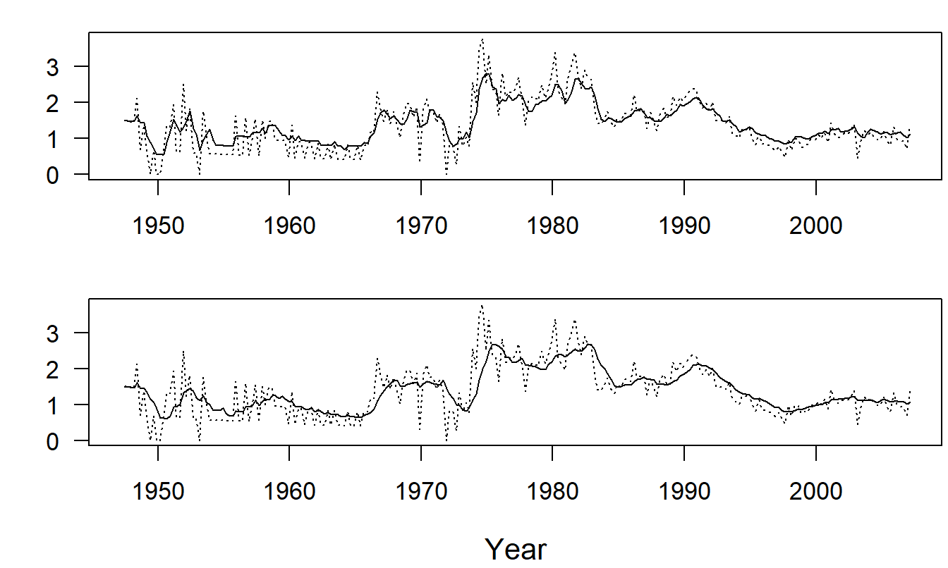
Figure 9.1: Quarterly Percentage Changes in the Medical Component of the Consumer Price Index. For both panels , the dashed line is the index. For the upper panel, the solid line is the smoothed version with \(k\)=4. For the lower panel, the solid line is the smoothed version with \(k\)=8. Source: Bureau of Labor Statistics
To forecast the series, re-express equation (9.1) recursively to get \[\begin{equation} \widehat{s}_t = \frac{y_t + y_{t-1} + \ldots + y_{t-k+1}}{k} = \frac{y_t + k \widehat{s}_{t-1} - y_{t-k}}{k} = \widehat{s}_{t-1} + \frac{y_t-y_{t-k}}{k}. \tag{9.2} \end{equation}\] If there are no trends in the data, then the second term on the right hand side, \((y_t-y_{t-k})/k\), may be ignored in practice. This yields the forecasting equation \(\widehat{y}_{T+l} = \widehat{s}_T\) for forecasts \(l\) lead time units into the future.
Several variants of running averages are available in the literature. For example, suppose that a series can be expressed as \(y_t = \beta_0 + \beta_1 t + \varepsilon_t\), a linear trend in time model. This can be handled through the following double smoothing procedure:
- Create a smoothed series using equation (9.1), that is, \(\widehat{s}_t^{(1)}=(y_t+\ldots+y_{t-k+1})/k.\)
- Create a doubly smoothed series by using equation (9.1) and treating the smoothed series created in step (i) as input. That is, \(\widehat{s}_t^{(2)} = (\widehat{s}_t^{(1)} + \ldots + \widehat{s}_{t-k+1}^{(1)})/k.\)
It is easy to check that this procedure smooths out the effect of a linear trend in time. The estimate of the trend is \(b_{1,T}=2\left( \widehat{s}_T^{(1)}-\widehat{s}_T^{(2)}\right) /(k-1)\). The resulting forecasts are \(\widehat{y}_{T+l} = \widehat{s}_T + b_{1,T}~l\) for forecasts \(l\) lead time units into the future.
Weighted Least Squares
An important feature of moving, or running, averages is that they can be expressed as weighted least squares (WLS) estimates. WLS estimation was introduced in Section 5.7.3. You will find additional broad discussion in Section 15.1.1. Recall that WLS estimates are minimizers of a weighted sum of squares. The WLS procedure is to find the values of \(b_0^{\ast}, \ldots, b_{k}^{\ast}\) that minimize
\[\begin{equation} WSS_T\left( b_0^{\ast },\ldots, b_k^{\ast}\right) = \sum_{t=1}^{T} w_t \left( y_t-\left( b_0^{\ast} + b_1^{\ast} x_{t1}, \ldots, b_{k}^{\ast} x_{tk} \right) \right)^2. \tag{9.3} \end{equation}\] Here, \(WSS_T\) is the weighted sum of squares at time \(T\).
To arrive at the moving, or running, average estimate, we use the model \(y_t = \beta_0 + \varepsilon_t\) with the choice of weights \(w_t=1\) for \(t = T-k+1, \ldots, T\) and \(w_t=0\) for \(t<T-k+1\). Thus, the problem of minimizing \(WSS_T\) in equation (9.3) reduces to finding \(b_0^{\ast}\) that minimizes \(\sum_{t=T-k+1}^{T}\left( y_t - b_0^{\ast} \right)^2.\) The value of \(b_0^{\ast}\) that this expression is \(b_0 = \widehat{s}_T\), which is the running average of length \(k\).
This model, together with this choice of weights, is called a locally constant mean model. Under a globally constant mean model, equal weights are used and the least squares estimate of \(\beta_0\) is the overall average, \(\overline{y}\). Under the locally constant mean model, we give equal weight to observations within \(k\) time units of the evaluation time \(T\) and zero weight to other observations. Although it is intuitively appealing to give more weight to more recent observations, the notion of an abrupt cut-off at a somewhat arbitrarily chosen \(k\) is not appealing. This criticism is addressed using exponential smoothing, introduced in the following section.
9.2 Exponential Smoothing
Exponential smoothing estimates are weighted averages of past values of a series, where the weights are given by a series that becomes exponentially small. To illustrate, think of \(w\) as a weight number that is between zero and one and consider the weighted average \[ \frac{y_t + w y_{t-1} + w^2 y_{t-2} + w^3 y_{t-3} + \ldots}{1/(1-w)}. \] This is a weighted average because the weights \(w^k (1-w)\) sum to one, that is, a geometric series expansion yields \(\sum_{k=0}^{\infty }w^k = 1/(1-w)\).
Because observations are not available in the infinite past, we use the truncated version \[\begin{equation} \widehat{s}_t = \frac{y_t + w y_{t-1} + \ldots + w^{t-1} y_1 + \ldots + w^t y_0}{1/(1-w) } \tag{9.4} \end{equation}\] to define the exponential smoothed estimate of the series. Here, \(y_0\) is the starting value of the series and is often chosen to be either zero, \(y_1\), or the average value of the series, \(\overline{y}\). Like running average estimates, the smoothed estimates in equation (9.4) provide greater weights to more recent observations as compared to observations far in the past with respect to time \(t\). Unlike running averages, the weight function is smooth.
The definition of exponential smoothing estimates in equation (9.4) appears complex. However, as with running averages in equation (9.2), we can re-express equation (9.4) recursively to yield \[\begin{equation} \widehat{s}_t = \widehat{s}_{t-1} + (1-w)(y_t-\widehat{s}_{t-1}) = (1-w) y_t + w \widehat{s}_{t-1}. \tag{9.5} \end{equation}\] The expression of the smoothed estimates in equation (9.5) is easier to compute than the definition in equation (9.4).
Equation (9.5) also provides insights into the role of \(w\) as the smoothing parameter. For example, on one hand as \(w\) gets close to zero, \(\widehat{s}_t\) gets close to \(y_t\). This indicates that little smoothing has taken place. On the other hand, as \(w\) gets close to one, there is little effect of \(y_t\) on \(\widehat{s}_t\). This indicates that a substantial amount of smoothing has taken place because the current fitted value is almost entirely composed of past observations.
Example: Medical Component of the CPI - Continued. To illustrate the effect of the choice of the smoothing parameter, consider the two panels of Figure 9.2. These are time series plots of the quarterly index of the medical component of the CPI. In the upper panel, the smoothed series with \(w=0.2\) is superimposed on the actual series. The lower panel is the corresponding graph with \(w=0.8\). From these figures, we can see that the larger is \(w\), the smoother are our fitted values.
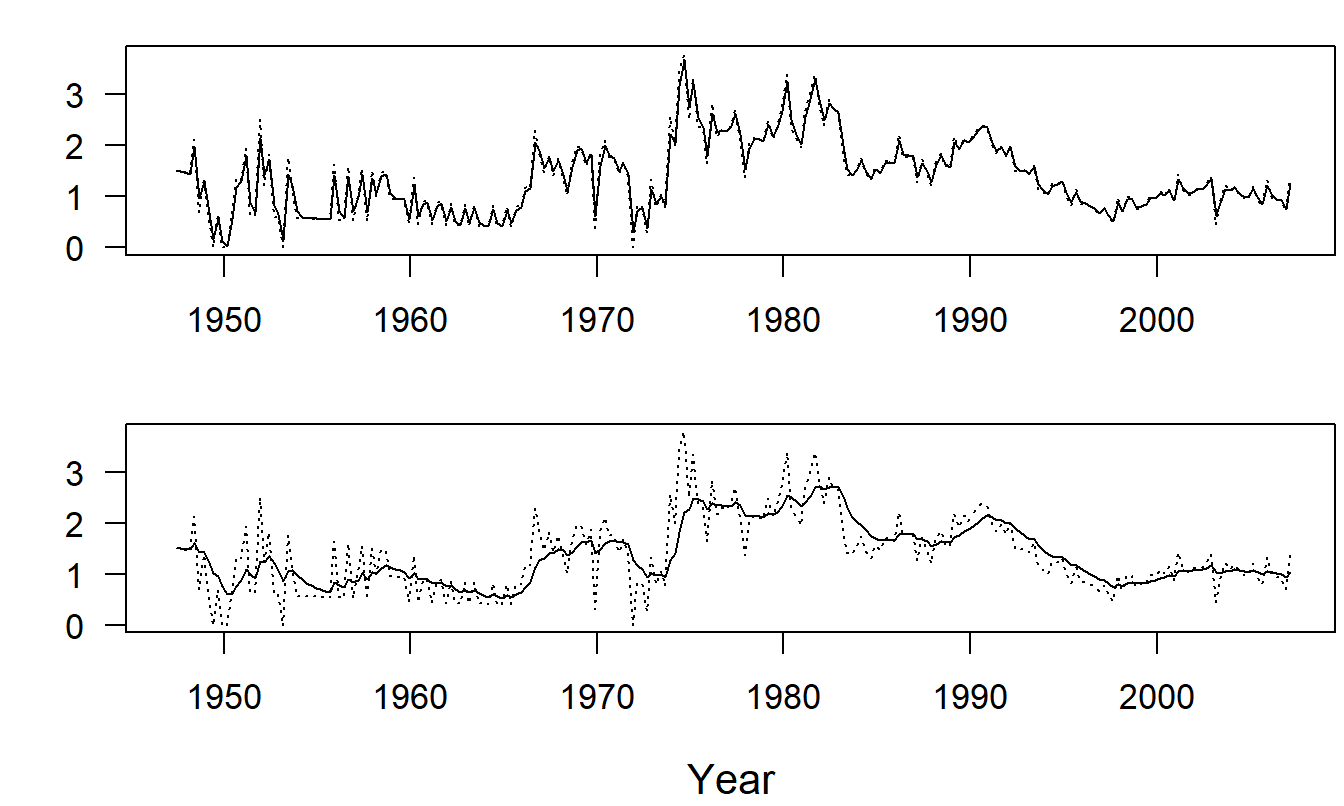
Figure 9.2: Medical Component of the Consumer Price Index with Smoothing. For both panels, the dashed line is the index. For the upper panel, the solid line is the smoothed version with \(w\)=0.2. For the lower panel, the solid line is the smoothed version with \(w\)=0.8.
Equation (9.5) also suggests using the relation \(\widehat{y}_{T+l} = \widehat{s}_T\) for our forecast of \(y_{T+l}\), that is, the series at \(l\) lead units in the future. Forecasts not only provide a way of predicting the future but also a way of assessing the fit. At time \(t-1\), our “forecast” of \(y_t\) is \(\widehat{s}_{t-1}\). The difference is called the one-step prediction error.
To assess the degree of fit, we use the sum of squared one-step prediction errors \[\begin{equation} SS\left( w\right) = \sum_{t=1}^T \left( y_t - \widehat{s}_{t-1} \right)^2. \tag{9.6} \end{equation}\] An important thing to note is that this sum of squares is a function of the smoothing parameter, \(w\). This then provides a criterion for choosing the smoothing parameter: choose the \(w\) that minimizes \(SS\left( w\right)\). Traditionally, analysts have recommended that \(w\) lie within the interval (.70, .95), without providing an objective criterion for the choice. Although minimizing \(SS\left( w\right)\) does provide an objective criterion, it is also computationally intensive. In absence of a sophisticated numerical routine, this minimization is typically accomplished by calculating \(SS\left( w\right)\) at a number of choices of \(w\) and choosing the \(w\) that provides the smallest value of \(SS\left( w\right)\).
To illustrate the choice of the exponential smoothing parameter \(w\), we return to the medical CPI example. Figure 9.3 summarizes the calculation of \(SS\left( w\right)\) for various values of \(w\). For this data set, it appears a choice of \(w \approx 0.50\) minimizes \(SS(w)\).
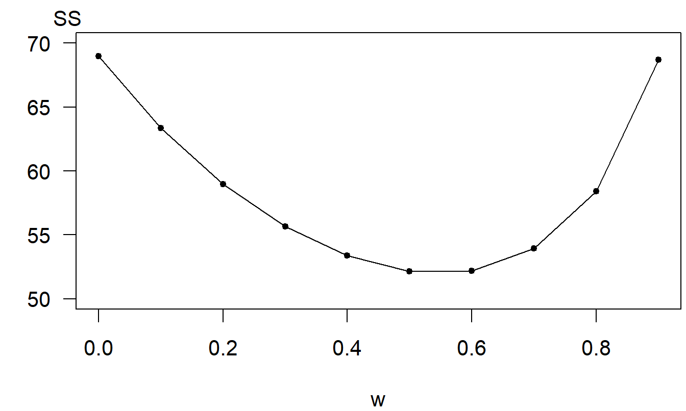
Figure 9.3: Sum of Squared One-Step Prediction Errors. Plot of the sum of squared prediction errors \(SS(w)\) as a function of the exponential smoothing parameter \(w\).
As with running averages, the presence of a linear trend in time, \(T_t = \beta_0 + \beta_1 t\), can be handled through the following double smoothing procedure:
- Create a smoothed series using equation (9.5), that is, \(\widehat{s}_t^{(1)} = (1-w) y_t + w \widehat{s}_{t-1}^{(1)}.\)
- Create a doubly smoothed series by using equation (9.5) and treating the smoothed series created in step (i) as input. That is, \(\widehat{s}_t^{(2)} = (1-w) \widehat{s}_t^{(1)} + w\widehat{s}_{t-1}^{(2)}\).
estimate of the trend is \(b_{1,T} = ((1-w)/w)(\widehat{s}_T^{(1)}- \widehat{s}_T^{(2)})\). The forecasts are given by \(\widehat{y}_{T+l}= b_{0,T}+b_{1,T}~l\) , where the estimate of the intercept is \(b_{0,T} = 2\widehat{s}_T^{(1)} - \widehat{s}_T^{(2)}\). We will also show how to use exponential smoothing for data with seasonal patterns in Section 9.3.
Weighted Least Squares
As with running averages, an important feature of exponentially smoothed estimates is that they can be expressed as WLS estimates. To see this, for the model \(y_t = \beta_0 + \varepsilon_t,\) the general weighted sum of squares in equation (9.3) reduces to \[ WSS_T\left( b_0^{\ast}\right) = \sum_{t=1}^T w_t \left( y_t - b_0^{\ast} \right)^2. \] The value of \(b_0^{\ast}\) that minimizes \(WSS_T\left( b_0^{\ast} \right)\) is \(b_0 = \left( \sum_{t=1}^T w_t y_t \right) / \left( \sum_{t=1}^T w_t \right)\). With the choice \(w_t = w^{T-t}\), we have \(b_0 \approx \widehat{s}_T\), where there is equality except for the minor issue of the starting value. Thus, exponential smoothing estimates are \(WLS\) estimates. Further, because of the choice of the form of the weights, exponential smoothing estimates are also called discounted least squares estimates. Here, \(w_t=w^{T-t}\) is a discounting function that one might use in considering the time value of money.
9.3 Seasonal Time Series Models
Seasonal patterns appear in many time series that arise in the study of business and economics. Models of seasonality are predominantly used to address patterns that arise as the result of an identifiable, physical phenomenon. For example, seasonal weather patterns affect people’s health and, in turn, the demand for prescription drugs. These same seasonal models may be used to model longer cyclical behavior.
There is a variety of techniques available for handling seasonal patterns including fixed seasonal effects, seasonal autoregressive models, and seasonal exponential smoothing methods. We address each of these techniques below.
Fixed Seasonal Effects
Recall that, in equations (7.1) and (7.2), we used \(S_t\) to represent the seasonal effects under additive and multiplicative decomposition models, respectively. A fixed seasonal effects model represents \(S_t\) as a function of time \(t\). The two most important examples are the seasonal binary and trigonometric functions. The Section 7.2 Trends in Voting Example showed how to use a seasonal binary variable and the Cost of Prescription Drugs Example below will demonstrate the use of trigonometric functions. The qualifier “fixed effects” means that relationships that are constant over time. In contrast, both exponential smoothing and autoregression techniques provide us with methods that adapt to recent events and allow for trends that change over time.
A large class of seasonal patterns can be represented using trigonometric functions. Consider the function \[ \mathrm{g}(t)=a\sin (ft+b) \] where \(a\) is the amplitude (the largest value of the curve), \(f\) is the frequency (the number of cycles that occurs in the interval \((0,2\pi )\)), and \(b\) is the phase shift. Because of a basic identity, \(\sin (x+y) = \sin x \cos y + \sin y \cos x\), we can write \[ \mathrm{g}(t) = \beta_1 \sin (ft) + \beta_2 \cos (ft) \] where \(\beta_1 = a \cos b\) and \(\beta_2 = a \sin b\). For a time series with seasonal base SB, we can represent a wide variety of seasonal patterns using \[\begin{equation} S_t = \sum_{i=1}^m a_i \sin (f_i t + b_i) = \sum_{i=1}^m \left\{ \beta_{1i} \sin (f_i t) + \beta_{2i} \cos (f_i t) \right\} \tag{9.7} \end{equation}\] with \(f_i=2\pi i/SB\). To illustrate, the complex function shown in Figure 9.5 was constructed as the sum of the \((m=)\) 2 simpler trigonometric functions that are shown in Figure 9.4.
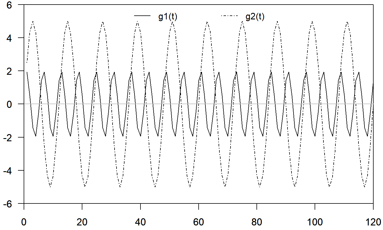
Figure 9.4: Plot of Two Trigonometric Functions. Here, g\(_1(t)\) has amplitude \(a_1=5\), frequency \(f_1=2 \pi /12\) and phase shift \(b_1=0\). Further, g\(_2(t)\) has amplitude \(a_2=2\), frequency \(f_2=4 \pi/12\) and phase shift \(b_2=\pi/4\).
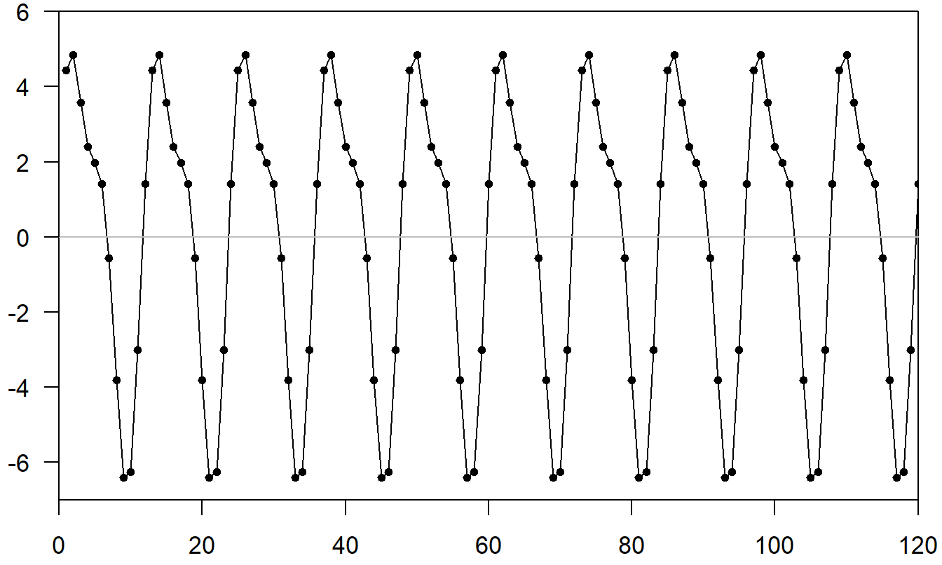
Figure 9.5: Plot of Sum of Two Trigonometric Functions in Figure 9.4.
Consider the model \(y_t=\beta_0+S_t+\varepsilon_t\), where \(S_t\) is specified in equation (9.7). Because \(\sin (f_it)\) and \(\cos (f_it)\) are functions of time, they can be treated as known explanatory variables. Thus, the model \[ y_t = \beta_0 + \sum_{i=1}^{m}\left\{ \beta_{1i}\sin (f_i t) + \beta_{2i} \cos (f_i t)\right\} + \varepsilon_t \] is a multiple linear regression model with \(k=2m\) explanatory variables. This model can be estimated using standard statistical regression software. Further, we can use our variable selection techniques to choose \(m\), the number of trigonometric functions. We note that \(m\) is at most \(SB/2\), for \(SB\) even. Otherwise, we would have perfect collinearity because of the periodicity of the sine function. The following example demonstrates how to choose \(m\).
Example: Cost of Prescription Drugs. We consider a series from the State of New Jersey’s Prescription Drug Program, the cost per prescription claim. This monthly series is available over the period August, 1986 through March, 1992, inclusive.
Figure 9.6 shows that the series is clearly nonstationary, in that cost per prescription claims are increasing over time. There are a variety of ways of handling this trend. One may begin with a linear trend in time and include lag claims to handle autocorrelations. For this series, a good approach to the modeling turns out to be to consider the percentage changes in the cost per claim series. Figure 9.7 is a time series plot of the percent changes. In this figure, we see that many of the trends that were evident in Figure 9.6 have been filtered out.
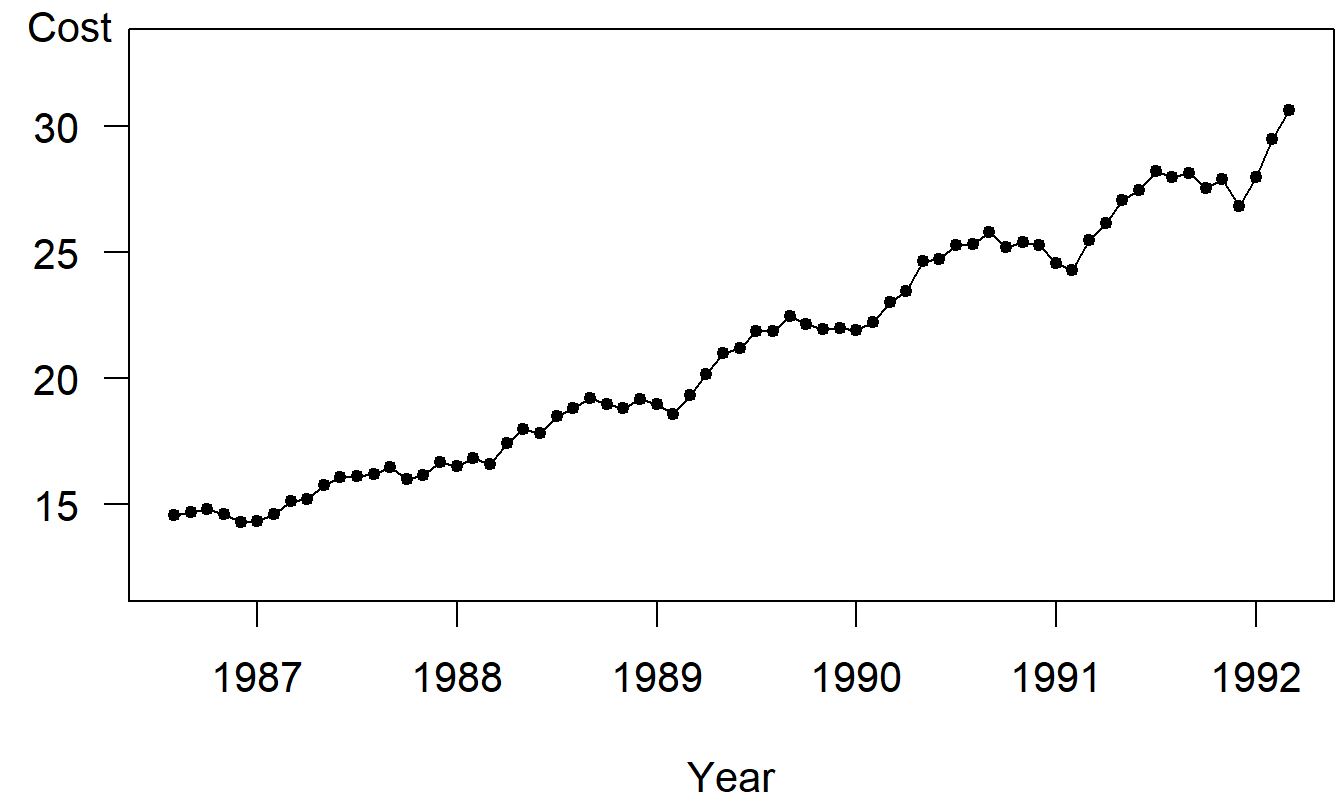
Figure 9.6: Time Series Plot of Cost per Prescription Claim of the State of New Jersey’s Prescription Drug Plan.
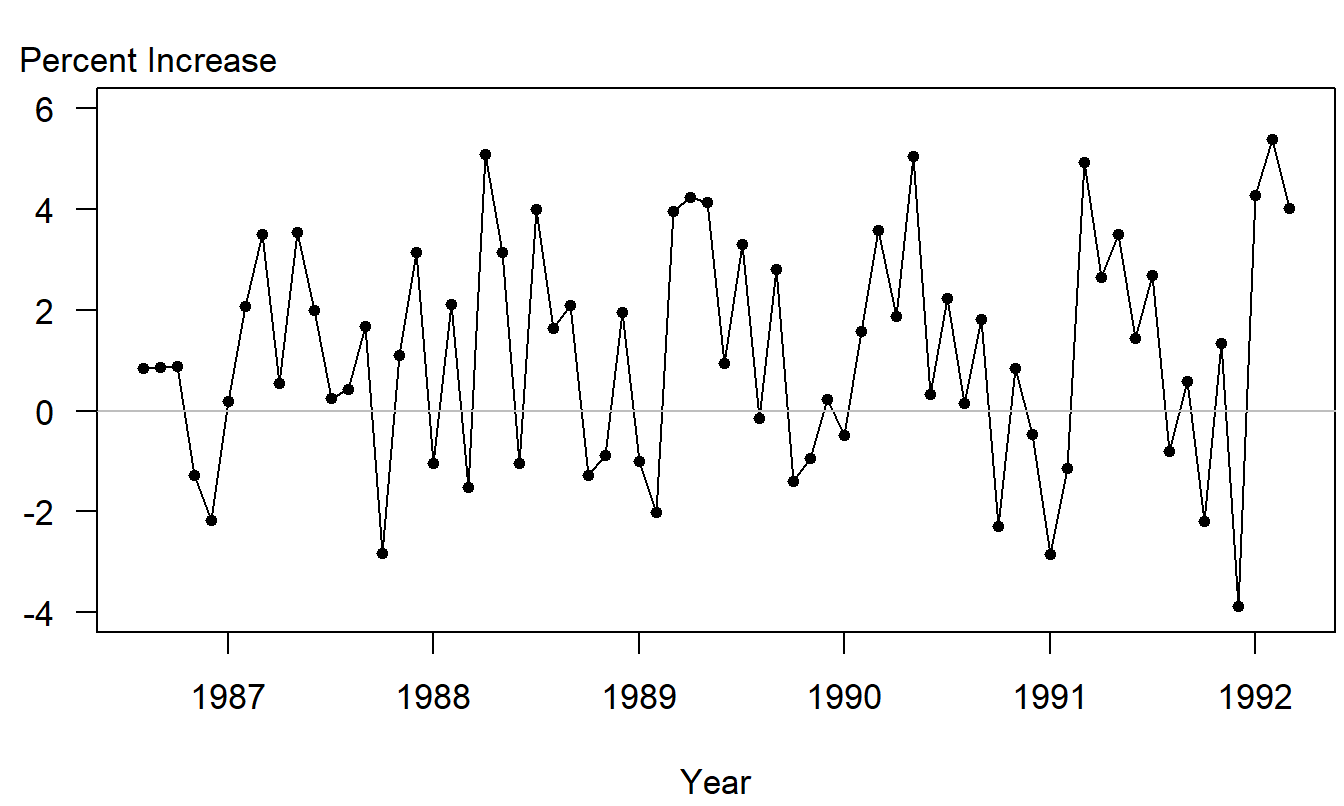
Figure 9.7: Monthly Percentage Changes of the Cost per Prescription Claim.
Figure 9.7 displays some mild seasonal patterns in the data. A close inspection of the data reveals higher percentage increases in the spring and lower increases in the fall months. A trigonometric function using \(m=1\) was fit to the data; the fitted model is \[ \begin{array}{cccc} \widehat{y}_t= & 1.2217 & -1.6956\sin (2\pi t/12) & +0.6536\cos (2\pi t/12) \\ {\small \text{std errors}} & {\small (0.2325)} & {\small (0.3269)} & {\small (0.3298)} \\ {\small t-\text{statistics}} & {\small [5.25]} & {\small [-5.08]} & {\small [1.98]} \end{array} \]
\(s=1.897\) and \(R^2=31.5\) percent. This model reveals some important seasonal patterns. The explanatory variables are statistically significant and an \(F\)-test establishes the significance of the model. Figure 9.8 shows the data with fitted values from the model superimposed. These superimposed fitted values help to detect visually the seasonal patterns.
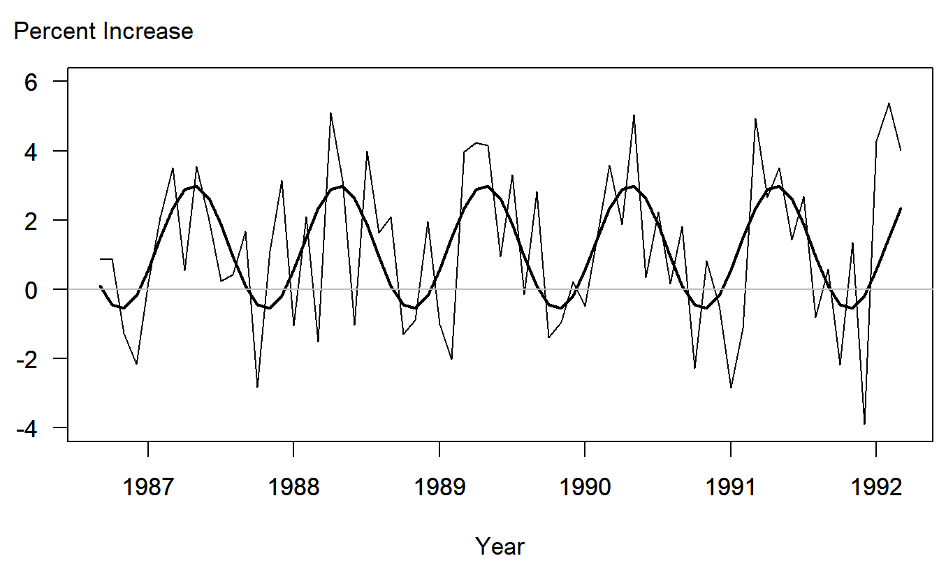
Figure 9.8: Monthly Percentage Changes of the Cost per Prescription claim. Fitted values from the seasonal trigonometric model have been superimposed.
Examination of the residuals from this fitted model revealed few further patterns. In addition, the model using \(m=2\) was fit to the data, resulting in \(R^2 = 33.6\) percent. We can decide whether to use \(m=1\) or \(2\) by considering the model \[ y_t = \beta_0 + \sum_{i=1}^2 \left\{ \beta_{1i} \sin (f_i t) + \beta_{2i} \cos (f_i t)\right\} + \varepsilon_t \] and testing \(H_0:\beta_{12} = \beta_{22}=0\). Using the partial \(F\)-test, with \(n=67, k=p=2\), we have \[ F-ratio=\frac{(0.336-0.315)/2}{(1.000-0.336)/62} = 0.98. \] With \(df_1=p=2\) and \(df_2=n-(k+p+1)=62\), the 95\(th\) percentile of the \(F\)-distribution is \(F\)-value = 3.15. Because \(F-ratio<F-value\), we can not reject \(H_0\) and conclude that \(m=1\) is the preferred choice.
Finally, it is also of interest to see how our model of the transformed data works with our original data, in units of cost per prescription claim. Fitted values of percentage increases were converted back to fitted values of cost per claim. Figure 9.9 shows the original data with fitted values superimposed. This figure establishes the strong relationship between the actual and fitted series.
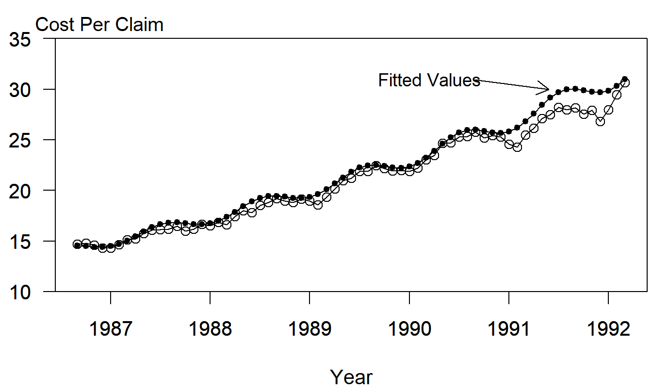
Figure 9.9: Monthly Percentage Changes of the Cost per Prescription Claim. Fitted values from the seasonal trigonometric model have been superimposed.
Seasonal Autoregressive Models
In Chapter 8 we examined patterns through time using autocorrelations of the form \(\rho_{k}\), the correlation between \(y_t\) and \(y_{t-k}\). We constructed representations of these temporal patterns using autoregressive models, regression models with lagged responses as explanatory variables. Seasonal time patterns can be handled similarly. We define the seasonal autoregressive model of order P, SAR(P), as \[\begin{equation} y_t=\beta_0+\beta_1y_{t-SB}+\beta_2y_{t-2SB}+\ldots+\beta _{P}y_{t-PSB}+\varepsilon_t, \tag{9.8} \end{equation}\] where \(SB\) is the seasonal base of under consideration. For example, using \(SB=12\), a seasonal model of order one, \(SAR(1)\), is \[ y_t=\beta_0+\beta_1y_{t-12}+\varepsilon_t. \] Unlike the \(AR(12)\) model defined in Chapter 9, for the \(SAR(1)\) model we have omitted \(y_{t-1},y_{t-2},\ldots,y_{t-11}\) as explanatory variables, although retaining \(y_{t-12}\).
Just as in Chapter 8, choice of the order of the model is accomplished by examining the autocorrelation structure and using an iterative model fitting strategy. Similarly, the choice of seasonality \(SB\) is based on an examination of the data. We refer the interested reader to Abraham and Ledolter (1983).
Example: Cost of Prescription Drugs - Continued. Table 9.1 presents autocorrelations for the percentage increase in cost per claim of prescription drugs. There are \(T=67\) observations for this data set, resulting in approximate standard error of \(se(r_{k})=1/\sqrt{67}\approx 0.122\). Thus, autocorrelations at and around lags 6, 12, and 18 appear to be different than zero. This suggests using \(SB=6\). Further examination of the data suggested a \(SAR(2)\) model.
Table 9.1. Autocorrelations of Cost per Prescription Claims
\[ \small{ \begin{array}{c|ccccccccc} \hline k & 1 & 2 & 3 & 4 & 5 & 6 & 7 & 8 & 9 \\ r_{k} & 0.08 & 0.10 & -0.12 & -0.11 & -0.32 & -0.33 & -0.29 & 0.07 & 0.08 \\ \hline k & 10 & 11 & 12 & 13 & 14 & 15 & 16 & 17 & 18 \\ r_{k} & 0.25 & 0.24 & 0.31 & -0.01 & 0.14 & -0.10 & -0.08 & -0.25 & -0.18 \\ \hline \end{array} } \]
The resulting fitted model is:
\[ \begin{array}{cccc} \widehat{y}_t= & 1.2191 & -0.2867y_{t-6} &+0.3120y_{t-12} \\ {\small \text{std errors}} & {\small (0.4064)} & {\small (0.1502)} & {\small (0.1489)} \\ {\small t-\text{statistics}} & {\small [3.00]} & {\small [-1.91]} & {\small [2.09]} \end{array} \]
\(s=2.156\). This model was fit using conditional least squares. Note that because we are using \(y_{t-12}\) as an explanatory variable, the first residual that can be estimated is 13. That is, we lose twelve observations when lagging by twelve when using least squares estimates.
Seasonal Exponential Smoothing
An exponential smoothing method that has enjoyed considerable popularity among forecasters is the Holt-Winter additive seasonal model. Although it is difficult to express forecasts from this model as a weighted least squares estimates, the model does appear to work well in practice.
Holt (1957) introduced the following generalization of the double exponential smoothing method. Let \(w_1\) and \(w_2\) be smoothing parameters and calculate recursively the parameter estimates:
\[\begin{eqnarray*} b_{0,t} &=&(1-w_1)y_t+w_1(b_{0,t-1}+b_{1,t-1}) \\ b_{1,t} &=&(1-w_2)(b_{0,t}-b_{0,t-1})+w_2b_{1,t-1} . \end{eqnarray*}\] These estimates can be used to forecast the linear trend model, \(y_t = \beta_0 + \beta_1 t + \varepsilon_t\). The forecasts are \(\widehat{y}_{T+l} = b_{0,T} + b_{1,T}~l\). With the choice \(w_1=w_2=2w/(1+w)\), the Holt procedure can be shown to produce the same estimates as the double exponential smoothing estimates described in Section 9.2. Because there are two smoothing parameters, the Holt procedure is a generalization of the doubly exponentially smoothed procedure. With two parameters, we need not use the same smoothing constants for the level (\(\beta_0\)) and the trend (\(\beta_1\)) components. This extra flexibility has found appeal with some data analysts.
Winters (1960) extended the Holt procedure to accommodate seasonal trends. Specifically, the Holt-Winter seasonal additive model is \[ y_t = \beta_0 + \beta_1 t + S_t + \varepsilon_t \] where \(S_t=S_{t-SB},S_1+S_2+\ldots+S_{SB}=0\), and \(SB\) is the seasonal base. We now employ three smoothing parameters: one for the level, \(w_1\), one for the trend, \(w_2\), and one for the seasonality, \(w_{3}\). The parameter estimates for this model are determined recursively using: \[\begin{eqnarray*} b_{0,t} &=&(1-w_1)\left( y_t-\widehat{S}_{t-SB}\right) +w_1(b_{0,t-1}+b_{1,t-1}) \\ b_{1,t} &=&(1-w_2)(b_{0,t}-b_{0,t-1})+w_2b_{1,t-1} \\ \widehat{S}_t &=&(1-w_{3})\left( y_t-b_{0,t}\right) +w_{3}\widehat{S} _{t-SB}. \end{eqnarray*}\] With these parameter estimates, forecasts are determined using: \[ \widehat{y}_{T+l}=b_{0,T}+b_{1,T}~l+\widehat{S}_T(l) \] where \(\widehat{S}_T(l)=\widehat{S}_{T+l}\) for \(l=1,2,\ldots,SB\), \(\widehat{S} _T(l)=\widehat{S}_{T+l-SB}\) for \(l=SB+1,\ldots,2SB\), and so on.
In order to compute the recursive estimates, we must decide on (i) initial starting values and (ii) a choice of smoothing parameters. To determine initial starting values, we recommend fitting a regression equation to the first portion of the data. The regression equation will include a linear trend in time, \(\beta_0 + \beta_1 t\), and \(SB-1\) binary variables for seasonal variation. Thus, only \(SB+1\) observations are required to determine initial estimates \(b_{0,0}, b_{1,0}, y_{1-SB}, y_{2-SB},\ldots, y_0\).
Choosing the three smoothing parameters is more difficult. Analysts have found it difficult to choose three parameters using an objective criterion, such as the minimization of the sum of squared one-step prediction errors, as in Section 9.2. Part of the difficulty stems from the nonlinearity of the minimization, resulting in prohibitive computational time. Another part of the difficulty is that functions such as the sum of squared one-step prediction errors often turn out to be relatively insensitive to the choice of parameters. Analysts have instead relied on rules of thumb to guide the choice of smoothing parameters. In particular, because seasonal effects may take several years to develop, a lower value of \(w_{3}\) is recommended (resulting in more smoothing). Cryer and Miller (1994) recommend \(w_1=w_2=0.9\) and \(w_{3}=0.6\).
9.4 Unit Root Tests
We have now seen two competing models that handle nonstationary with a mean trend, the linear trend in time model and the random walk model. Section 7.6 illustrated how we can choose between these two models on a out-of-sample basis. For a selection procedure based on in-sample data, consider the model \[ y_t = \mu_0 + \phi (y_{t-1} - \mu_0) + \mu_1 \left( \phi + (1-\phi) t \right) + \varepsilon_t. \] When \(\phi =1\), this reduces to a random walk model with \(y_t=\mu_1+y_{t-1}+\varepsilon_t.\) When \(\phi <1\) and \(\mu_1=0\), this reduces to an \(AR(1)\) model, \(y_t=\beta_0+\phi y_{t-1}+\varepsilon_t\), with \(\beta_0=\mu_0\left( 1-\phi \right)\). When \(\phi =0\), this reduces to a linear trend in time model with \(y_t = \mu_0 + \mu_1 t + \varepsilon_t.\)
Running a model where the left-hand side variable is potentially a random walk is problematic. Hence, it is customary to use least squares on the model \[\begin{equation} y_t-y_{t-1}=\beta_0+\left( \phi -1\right) y_{t-1}+\beta _1t+\varepsilon_t \tag{9.9} \end{equation}\] where we interpret \(\beta_0=\mu_0\left( 1-\phi \right) + \phi \mu_1\) and \(\beta_1=\mu_1\left( 1-\phi \right).\) From this regression, let $ t_{DF}$ be the \(t\)-statistic associated with the \(y_{t-1}\) variable. We wish to use the \(t\)-statistic to test the null hypothesis that \(H_0:\phi =1\) versus the one-sided alternative that \(H_{a}:\phi <1\). Because \(\{y_{t-1}\}\) is a random walk process under the null hypothesis, the distribution of \(t_{DF}\) does not follow the usual \(t\)-distribution but rather follows a special distribution, due to Dickey and Fuller (1979). This distribution has been tabulated has been programmed in several statistical packages, Fuller (1996).
Example: Labor Force Participation Rates - Continued. We illustrate the performance of the Dickey-Fuller tests on the labor force participation rates introduced in Chapter 7. There, we established that the series was clearly non-stationary and that out-of-sample forecasting showed the random walk to be preferred when compared to the linear trend in time model.
Table 9.2 summarizes the test. Both without (\(\mu_1 = 0\)) and with (\(\mu_1 \neq 0\)) the trend line, the \(t\)-statistic (\(t_{DF}\)) is statistically insignificant (compared to the 10% critical value). This provides evidence that the random walk is the preferred model choice.
Table 9.2. Dickey-Fuller Test Statistics with Critical Values
\[ \small{ \begin{array}{c|cccc} \hline & \text{Without Trend} & &\text{With Trend} \\ & & 10\% ~ \text{Critical} & & 10\%~ \text{Critical} \\ \text{Lag} (p)& t_{DF} & \text{Value} & t_{DF} & \text{Value} \\ \hline & -1.614 & -2.624 & -0.266 & -3.228 \\ 1 & -1.816 & -2.625 & -0.037 & -3.230 \\ 2 & -1.736 & -2.626 & 0.421 & -3.233 \\ \hline \end{array} } \]
One criticism of the Dickey-Fuller test is that the disturbance term
in equation (9.9) is presumed to be serially
uncorrelated. To protect against this, a commonly used alternative
is the augmented Dickey-Fuller test statistic. This is the
\(t\)-statistic associated with the \(y_{t-1}\) variable using ordinary
least squares on the following equation
\[\begin{equation}
y_t-y_{t-1}=\beta_0+\left( \phi -1\right) y_{t-1}+\beta
_1t+\sum_{j=1}^{p}\phi_{j}\left( y_{t-j}-y_{t-j-1}\right)
+\varepsilon_t.
\tag{9.10}
\end{equation}\]
In this equation, we have augmented the disturbance term by
autoregressive terms in the differences {\(y_{t-j}-y_{t-j-1}\)}.
The idea is that these terms serve to capture serial correlation in
the disturbance term. Research has not reached consensus on how to
choose the number of lags (\(p\)) - in most applications, analysts
provide results of the test statistic for a number of choices of
lags and hope that conclusions reached are qualitatively similar.
This is certainly the case for the labor force participation rates
as demonstrated in Table 9.2. Here, we see that for
each lag choice, the random walk null hypothesis can not be
rejected.
9.5 ARCH/GARCH Models
To this point, we have focused on forecasting the level of the series - that is, the conditional mean. However, there are important applications, notably in the study of finance, where forecasting the variability is important. To illustrate, the variance plays a key role in option pricing, such as when using the Black-Scholes formula.
Many financial time series exhibit volatility clustering, that is, periods of high volatility (large changes in the series) followed by periods of low volatility. To illustrate, consider the following.
Example: S & P 500 Daily Returns. Figure 9.10 provides a time series plot of daily returns from the Standard & Poor’s 500 over the period 2000-2006, inclusive. Here, we see the early part of the series, prior to January of 2003 is more volatile when compared to the latter part of the series. Except for the changing volatility, the series appears to be stationary, without dramatic increases or decreases.
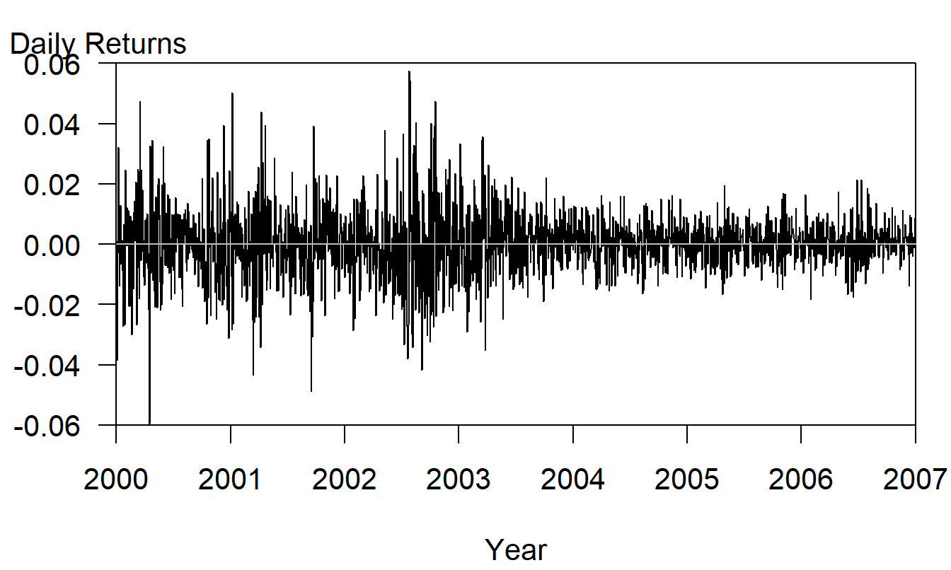
Figure 9.10: Time Series Plot of Daily S&P Returns, 2000-2006, inclusive.
The concept of variability changing over time seems at odds with our notions of stationarity. This is because a condition for weak stationary is that the series has a constant variance. The surprising thing is that we can allow for changing variances by conditioning on the past and still retain a weakly stationary model. To see this mathematically, we use the notation \(\Omega_t\) to denote the information set, the collection of knowledge about the process up to and including time \(t\). For a weakly stationary series, we may denote this as \(\Omega _t=\{\varepsilon_t,\varepsilon_{t-1},\ldots\}\). We allow the variance to depend on time \(t\) by conditioning on the past, \[ \sigma_t^2=\mathrm{Var}_{t-1}\left( \varepsilon_t\right) =\mathrm{E} \left( \left[ \varepsilon_t-\mathrm{E}\left( \varepsilon_t|\Omega _{t-1}\right) \right] ^2|\Omega_{t-1}\right) . \] We now present several parametric models of \(\sigma_t^2\) that allows us to quantify and forecast this changing volatility.
ARCH Model
The autoregressive changing heteroscedasticity model of order p, \(ARCH(p),\) is due to Engle (1982). We now assume that the distribution of \(\varepsilon_t\) given \(\Omega_{t-1}\) is normally distributed with mean zero and variance \(\sigma_t^2\). We further assume that the conditional variance is determined recursively by \[ \sigma_t^2=w+\gamma_1\varepsilon_{t-1}^2+\ldots+\gamma _{p}\varepsilon_{t-p}^2=w+\gamma (B)\varepsilon_t^2, \] where \(\gamma (x)=\gamma_1x+\ldots+\gamma_{p}x^{p}.\) Here, \(w>0\) is the “long-run” volatility parameter and $ _1,,_p$ are coefficients such that \(\gamma _j \geq 0\) and \(\gamma (1)=\sum_{j=1}^{p} \gamma_j < 1\).
In the case that \(p=1\), we can see that a large change to the series $ _{t-1}^2\(\ can induce a large conditional variance\)_t^2$. Higher orders of \(p\) help capture longer term effects. Thus, this model is intuitively appealing to analysts. Interestingly, Engle provided additional mild conditions to assure that the \(\{\varepsilon_t\}\) is weakly stationarity. Thus, despite having a changing conditional variance, the unconditional variance remains constant over time.
GARCH Model
The generalized ARCH model of order p, \(GARCH(p,q),\) complements the \(ARCH\) model in the same way that the moving average complements the autoregressive model. As with the \(ARCH\) model, we assume that the distribution of \(\varepsilon_t\) given \(\Omega_{t-1}\) is normally distributed with mean zero and variance \(\sigma_t^2\). The conditional variance is determined recursively by \[ \sigma_t^2-\delta_1\sigma_{t-1}^2+-\ldots-\delta_{q}\sigma _{t-q}^2=w+\gamma_1\varepsilon_{t-1}^2+\ldots+\gamma_{p}\varepsilon _{t-p}^2, \] or \(\sigma_t^2=w+\gamma (B)\varepsilon_t^2+\delta (B)\sigma_t^2,\) where \(\delta (x)=\delta_1x+\ldots+\delta_{q}x^{q}.\) In addition to the \(ARCH(p)\) requirements, we also need \(\delta_{j}\geq 0\) and \(\gamma (1)+\delta \left( 1\right) <1\).
As it turns out, the \(GARCH(p,q)\) is also a weakly stationary model, with mean zero and (unconditional) variance \(\mathrm{Var~}\varepsilon_t=w/(1-\gamma (1)-\delta \left( 1\right) ).\)
Example: S & P 500 Daily Returns - Continued. After an examination of the data (details not given here), an \(MA(2\)) model was fit to the series with \(GARCH(1,1)\) errors. Specifically, if \(y_t\) denotes the daily return from the S & P series, for \(t=1,\ldots,1759\), we fit the model \[ y_t = \beta_0 + \varepsilon_t - \theta_1 \varepsilon_{t-1} - \theta_2 \varepsilon_{t-2}, \] where the conditional variance is determined recursively by \[ \sigma_t^2 - \delta_1 \sigma_{t-1}^2 = w + \gamma_1 \varepsilon_{t-1}^2. \]
The fitted model appears in Table 9.3. Here, the statistical package we used employs maximum likelihood to determine the estimated parameters as well as the standard errors needed for the \(t\)-statistics. The \(t\)-statistics show that all parameter estimates, except \(\theta_1\), are statistically significant. As discussed in Chapter 8, the convention is to retain lower order coefficients, such as \(\theta_1\), if higher order coefficients like \(\theta_2\) are significant. Note from Table 9.3 that the sum of the \(ARCH\) coefficient (\(\delta_1\)) and the \(GARCH\) coefficient (\(\gamma_1\)) are nearly one with \(GARCH\) coefficient substantially larger than the \(ARCH\) coefficient. This phenomenon is also reported by Diebold (2004, page 400) who states that it is commonly found in studies of financial asset returns.
Table 9.3. S & P 500 Daily Returns Model Fit
\[ \small{ \begin{array}{crr} \hline \text{Parameter} & \text{Estimate} & t-\text{statistic} \\ \hline \beta_0 & 0.0004616 & 2.51 \\ \theta_1 & -0.0391526 & -1.49 \\ \theta_2 & -0.0612666 & -2.51 \\ \delta_1 & 0.0667424 & 6.97 \\ \gamma_1 & 0.9288311 & 93.55 \\ w & 5.61\times 10^{-7} & 2.30 \\ \text{Log-likelihood} & 5,658.852 & \\ \hline \end{array} } \]
9.6 Further Reading and References
For other variations of the running average method and exponential smoothing, see Abraham and Ledolter (1983).
For a more detailed treatment of unit root tests, we refer the reader to Diebold (2004) or Fuller (1996) for a more advanced treatment.
Chapter References
- Abraham, Bovas and Ledolter, Johannes (1983). Statistical Methods for Forecasting. John Wiley & Sons, New York.
- Cryer, Jon D. and Robert B. Miller (1994). Statistics for Business: Data Analysis and Modelling. PWS-Kent, Boston.
- Dickey, D. A. and Wayne A. Fuller (1979). Distribution of the estimators for autoregressive time series with a unit root. Journal of the American Statistical Association 74, 427-431.
- Diebold, Francis X. (2004). Elements of Forecasting , Third Edition. Thomson, South-Western, Mason Ohio.
- Engle, R. F. (1982). Autoregressive conditional heteroscedasticity with estimates of UK inflation. Econometrica 50, 987-1007.
- Fuller, Wayne A. (1996). Introduction to Statistical Time Series, Second Edition. John Wiley & Sons, New York.
- Holt, C. C. (1957). Forecasting trends and seasonals by exponenetially weighted moving averages. O.N.R. Memorandum, No. 52, Carnegie Institute of Technology.
- Winters, P. R. (1960). Forecasting sales by exponentially weighted moving averages. Management Science 6, 324-342.