Chapter 13 Generalized Linear Models
Chapter Preview. This chapter describes a unifying framework for the Part I linear model and the binary and count models in Chapters 11 and 12. Generalized linear models, often known by the acronym GLM, represent an important class of nonlinear regression models that have found extensive use in actuarial practice. This unifying framework not only encompasses many models we have seen but also provides a platform for new ones, including gamma regressions for fat-tailed data and “Tweedie” distributions for two-part data.
13.1 Introduction
There are many ways to extend, or generalize, the linear regression model. This chapter introduces an extension that is so widely used that it is known as the “generalized linear model,” or as the acronym GLM.
Generalized linear models include linear, logistic and Poisson regressions, all as special cases. One common feature of these models is that in each case we can express the mean response as a function of linear combinations of explanatory variables. In the GLM context, it is customary to use \(\mu_i = \mathrm{E}~y_i\) for the mean response and call \(\eta_i = \mathbf{x}_i^{\mathbf{\prime}} \boldsymbol \beta\) the systematic component of the model. We have seen that we can express the systematic component as:
- \(\mathbf{x}_i^{\mathbf{\prime}}\boldsymbol \beta = \mu_i\), for (normal) linear regression,
- \(\mathbf{x}_i^{\mathbf{\prime}} \boldsymbol \beta = \exp(\mu_i)/(1+\exp(\mu_i)),\) for logistic regression and
- \(\mathbf{x}_i^{\mathbf{\prime}} \boldsymbol \beta = \ln (\mu_i),\) for Poisson regression.
For GLMs, the systematic component is related to the mean through the expression \[\begin{equation} \eta _i = \mathbf{x}_i^{\mathbf{\prime}} \boldsymbol \beta = \mathrm{g}\left( \mu _i\right). \tag{13.1} \end{equation}\] Here, g(.) is known and called the link function. The inverse of the link function, \(\mu _i = \mathrm{g}^{-1}( \mathbf{x}_i^{\mathbf{\prime}} \boldsymbol \beta)\), is the mean function.
The second common feature involves the distribution of the dependent variables. In Section 13.2, we will introduce the linear exponential family of distributions, an extension of the exponential distribution. This family includes the normal, Bernoulli and Poisson distributions as special cases.
The third common feature of GLM models is the robustness of inference to the choice of distributions. Although linear regression is motivated by normal distribution theory, we have seen that responses need not be normally distributed for statistical inference procedures to be effective. The Section 3.2 sampling assumptions focus on:
- the form of the mean function (assumption F1),
- non-stochastic or exogenous explanatory variables (F2),
- constant variance (F3) and
- independence among observations (F4).
GLM models maintain assumptions F2 and F4 and generalize F1 through the link function. The choice of different distributions allows us to relax F3 by specifying the variance to be a function of the mean, written as \(\mathrm{Var~}y_i = \phi v(\mu_i)\). Table 13.1 shows how the variance depends on the mean for different distributions. As we will see when considering estimation (Section 13.3), it is the choice of the variance function that drives the most important inference properties, not the choice of the distribution.
Table 13.1. Variance Functions for Selected Distributions
\[ \small{ \begin{array}{lc} \hline \text{Distribution} & \text{Variance Function }v(\mu) \\ \hline \text{Normal} & 1 \\ \text{Bernoulli} & \mu ( 1- \mu ) \\ \text{Poisson} & \mu \\ \text{Gamma }& \mu ^2 \\ \text{Inverse Gaussian} & \mu ^3 \\ \hline \end{array} } \]
By considering regression in the GLM context, we will be able to handle dependent variables that are approximately normally distributed, binary or representing counts, all within one framework. This will aid our understanding of regression by allowing us to see the “big picture” and not be so concerned with the details. Further, the generality of GLMs will allow us to introduce new applications, such as gamma regressions that are useful for fat-tailed distributions and the so-called “Tweedie” distributions for two-part data. Two-part data is a topic taken up in Chapter 16, where there is a mass at zero and a continuous component. For insurance claims data, the zero represents no claim and the continuous component represents the amount of a claim.
This chapter describes estimation procedures for calibrating GLM models, significance tests and goodness of fit statistics for documenting the usefulness of the model, and residuals for assessing the robustness of the model fit. We will see that the our earlier work done on linear, binary and count regression models provides the foundations for the tools needed for the GLM model. Indeed, many are slight variations of tools and concepts developed earlier in this text and we will be able to build on these foundations.
Video: Section Summary
13.2 GLM Model
To specify a GLM, the analyst chooses an underlying response distribution, the topic of Section 13.2.1, and a function that links the mean response to the covariates, the topic of Section 13.2.2.
13.2.1 Linear Exponential Family of Distributions
Definition. The distribution of the linear exponential family is \[\begin{equation} \mathrm{f}( y; \theta ,\phi ) =\exp \left( \frac{y\theta -b(\theta )}{\phi } +S\left( y,\phi \right) \right). \tag{13.2} \end{equation}\] Here, \(y\) is a dependent variable and \(\theta\) is the parameter of interest. The quantity \(\phi\) is a scale parameter. The term \(b(\theta )\) depends only on the parameter \(\theta\), not the dependent variable. The statistic \(S\left( y,\phi \right)\) is a function of the dependent variable and the scale parameter, not the parameter \(\theta\).
The dependent variable \(y\) may be discrete, continuous or a mixture. Thus, \(\mathrm{f} \left( .\right)\) may be interpreted to be a density or mass function, depending on the application. Table 13.8 provides several examples, including the normal, binomial and Poisson distributions. To illustrate, consider a normal distribution with a probability density function of the form \[\begin{eqnarray*} \mathrm{f}( y; \mu ,\sigma ^{2}) &=&\frac{1}{\sigma \sqrt{2\pi }}\exp \left( - \frac{(y-\mu )^{2}}{2\sigma ^{2}}\right) \\ &=&\exp \left( \frac{(y\mu -\mu ^{2}/2)}{\sigma ^{2}}-\frac{y^{2}}{2\sigma ^{2}}-\frac{1}{2}\ln \left( 2\pi \sigma ^{2}\right) \right) . \end{eqnarray*}\] With the choices \(\theta =\mu\), \(\phi =\sigma ^{2}\), \(b(\theta )=\theta ^{2}/2\) and \(S\left( y,\phi \right) =-y^{2}/(2\phi )-\ln \left( 2\pi \phi \right) /2\), we see that the normal probability density function can be expressed as in equation (13.2).
For the distribution in equation (13.2), some straightforward calculations show that
- \(\mathrm{E~}y=b^{\prime }(\theta )\) and
- \(\mathrm{Var~}y=\phi b^{\prime \prime }(\theta )\).
For reference, these calculations appear in Section 13.9.2. To illustrate, in the context of the normal distribution example above, it is easy to check that \(\mathrm{E~}y=b^{\prime }(\theta )=\theta =\mu\) and \(\mathrm{Var~} y = \sigma ^{2}b^{\prime \prime }(\theta )=\sigma ^{2}\), as anticipated.
In regression modeling situations, the distribution of \(y_i\) varies by observation through the subscript “\(i\)”. It is customary to let the distribution family remain constant yet allow the parameters to vary by observation through the notation \(\theta_i\) and \(\phi_i\). For our applications, the variation of the scale parameter is due to known weight factors. Specifically, when the scale parameter varies by observation, it is according to \(\phi _i=\phi /w_i\), that is, a constant divided by a known weight \(w_i\). With the relation \(\mathrm{Var~}y_i=\phi_i b^{\prime \prime }(\theta_i)=\phi b^{\prime \prime }(\theta_i)/w_i\), we have that a larger weight implies a smaller variance, other things being equal.
13.2.2 Link Functions
In regression situations, we wish to understand the impact of \(\eta_i = \mathbf{x}_i^{\mathbf{\prime}} \boldsymbol \beta\), the systematic component. As we saw in the prior subsection, we can express the mean of \(y_i\) as \(\mathrm{E~}y_i=\mu _i=b^{\prime }(\theta_i)\). Equation (13.1) serves to “link” the systematic component to \(\mu_i\) and thus to the parameter \(\theta_i\). It is possible to use the identity function for g(.) so that \(\mu _i=b^{\prime }(\theta_i)\). Indeed, this is the usual case in linear regression. However, linear combinations of explanatory variables, \(\mathbf{x}_i^{\mathbf{\prime }}\boldsymbol \beta\), may vary between negative and positive infinity whereas means are often restricted to smaller range. For example, Poisson means vary between zero and infinity. The link function serves to map the domain of the mean function onto the whole real line.
Special Case: Links for the Bernoulli distribution. Bernoulli means are probabilities and thus vary between zero and one. For this case, it is useful to choose a link function that maps the unit interval (0,1) onto the whole real line. The following are three important examples of link functions for the Bernoulli distribution:
- Logit: \(g(\mu )=\mathrm{logit}(\mu )=\ln (\mu /(1-\mu ))\) .
- Probit: \(g(\mu )=\Phi ^{-1}(\mu )\), where \(\Phi ^{-1}\) is the inverse of the standard normal distribution function.
- Complementary log-log: \(g(\mu )=\ln \left( -\ln (1-\mu )\right)\).
This illustration demonstrates that there may be several link functions that are suitable for a particular distribution. To help with the selection, an intuitively appealing case occurs when the systematic component equals the parameter of interest ($=$). To see this, first recall that $ =g()$ and \(\mu =b^{\prime }(\theta )\), dropping the “\(i\)” subscripts for the moment. Then, it is easy to see that if \(g^{-1}=b^{\prime }\), then \(\eta =g(b^{\prime }(\theta ))=\theta\). The choice of \(g\) that is the inverse of \(b^{\prime }(\theta )\) is called the canonical link.
Table 13.2 shows the mean function and corresponding canonical link for several important distributions.
Table 13.2. Mean Functions and Canonical Links for Selected Distributions
\[ \small{ \begin{array}{lcc} \hline \text{Distribution} & \text{Mean function } b^{\prime }(\theta ) & \text{Canonical link }g(\mu ) \\ \hline \text{Normal} & \theta & \mu \\ \text{Bernoulli} & e^{\theta}/(1+e^{\theta} ) & \mathrm{logit}(\mu ) \\ \text{Poisson} & e^{\theta } & \ln \mu \\ \text{Gamma} & -1/\theta & -1/\mu \\ \text{Inverse Gaussian} & (-2 \theta )^{-1/2} & -1 /(2 \mu^2) \\ \hline \end{array} } \]
Links relate the mean to the systematic component and to the regression parameters. Because the regression parameters are unknown, it is common to specify the links only up to scale. For example, it is common to specify the inverse gaussian canonical link as \(1 /\mu^2\) (instead of $-1 /(2 ^2) $). If necessary, one can always recover the scale when estimating the unknown regression coefficients.
Example: Ratemaking Classification. The process of grouping risks with similar characteristics is known as risk classification. Ratemaking is the art of setting premiums, or rates, based on loss experience and exposures of risk classes. For example, Mildenhall (1999) considered 8,942 collision losses from private passenger United Kingdom (UK) automobile insurance policies. The data were derived from Nelder and McCullagh (1989, Section 8.4.1) but originated from Baxter et al. (1980). A typical personal auto rating plan is based on driver and vehicle characteristics. Driver characteristics may include the driver’s age, gender, marital status, history (accidents and violations) and good student discount. Vehicle characteristics may include vehicle model type and year, purpose (business/school or pleasure), garage territory and so forth. We can represent the systematic component as \[ \eta_{ij} = \beta_0 + \alpha_i + \tau_j, \] where \(\alpha_i\) represents the effect of the \(i\)th category of driver classification and \(\tau_j\) the effect of the \(j\)th vehicle type. Table 13.3 displays the Mildenhall data for eight driver types (age groups) and four vehicle classes (vehicle use). The average severity is in pounds sterling adjusted for inflation.
In GLM terminology, an additive rating plan is based on the identity link function whereas a multiplicative plan is based on a logarithmic link function. Specifically, if we use \(\eta_{ij} = \ln ( \mu _{ij})\), then we can write the mean as \[\begin{equation} \mu _{ij} = \exp(\beta_0 + \alpha_i + \tau_j) = B \times A_i \times T_j, \tag{13.3} \end{equation}\] where \(B=\exp(\beta_0)\) is a scaling constant, \(A_i=\exp(\alpha_i)\) represents driver effects and \(T_j=\exp(\tau_j)\) represents vehicle effects.
Table 13.3. Private Passenger Automobile UK Collision Data
\[ \small{ \begin{array}{lcrr|llcrr} \hline \text{Age} & \text{Vehicle} & \text{ Average} & \text{Claim} &~~~ & \text{Age} & \text{Vehicle} & \text{ Average} & \text{Claim} \\ \text{Group} & \text{Use} & \text{Severity} & \text{Count} & & \text{Group} & \text{Use} & \text{Severity} & \text{Count} \\ \hline 17-20 & \text{Pleasure} & 250.48 & 21 & & 35-39 & \text{Pleasure} & 153.62 & 151 \\ 17-20 & \text{DriveShort} & 274.78 & 40 & & 35-39 & \text{DriveShort} & 201.67 & 479 \\ 17-20 & \text{DriveLong} & 244.52 & 23 & & 35-39 & \text{DriveLong} & 238.21 & 381 \\ 17-20 & \text{Business} & 797.80 & 5 & & 35-39 & \text{Business} & 256.21 & 166 \\ \hline 21-24 & \text{Pleasure} & 213.71 & 63 & & 40-49 & \text{Pleasure} & 208.59 & 245 \\ 21-24 & \text{DriveShort} & 298.60 & 171 & & 40-49 & \text{DriveShort} & 202.80 & 970 \\ 21-24 & \text{DriveLong} & 298.13 & 92 & & 40-49 & \text{DriveLong} & 236.06 & 719 \\ 21-24 & \text{Business} & 362.23 & 44 & & 40-49 & \text{Business} & 352.49 & 304 \\ \hline 25-29 & \text{Pleasure} & 250.57 & 140 & & 50-59 & \text{Pleasure} & 207.57 & 266 \\ 25-29 & \text{DriveShort} & 248.56 & 343 & & 50-59 & \text{DriveShort} & 202.67 & 859 \\ 25-29 & \text{DriveLong} & 297.90 & 318 & & 50-59 & \text{DriveLong} & 253.63 & 504 \\ 25-29 & \text{Business} & 342.31 & 129 & & 50-59 & \text{Business} & 340.56 & 162 \\ \hline 30-34 & \text{Pleasure} & 229.09 & 123 & & 60+ & \text{Pleasure} & 192.00 & 260 \\ 30-34 & \text{DriveShort} & 228.48 & 448 & & 60+ & \text{DriveShort} & 196.33 & 578 \\ 30-34 & \text{DriveLong} & 293.87 & 361 & & 60+ & \text{DriveLong} & 259.79 & 312 \\ 30-34 & \text{Business} & 367.46 & 169 & & 60+ & \text{Business} & 342.58 & 96 \\ \hline \end{array} } \] Source: Mildenhall (1999). “DriveShort” means drive to work but less than 10 miles.”DriveLong” means drive to work but more than 10 miles.
R Code to Produce Table 13.3
Video: Section Summary
13.3 Estimation
This section presents maximum likelihood, the customary form of estimation. To provide intuition, we focus on the simpler case of canonical links. Results for more general links appear in Section 13.9.3.
13.3.1 Maximum Likelihood Estimation for Canonical Links
From equation (13.2) and the independence among observations, the log-likelihood is \[\begin{equation} \ln \mathrm{f}( \mathbf{y}) =\sum_{i=1}^n \left\{ \frac{y_i\theta_i-b(\theta_i)}{\phi _i}+S( y_i,\phi _i ) \right\} . \tag{13.4} \end{equation}\] Recall that for canonical links, we have equality between the distribution’s parameter and the systematic component, so that \(\theta_i=\eta _i=\mathbf{x}_i^{\mathbf{\prime }}\boldsymbol \beta\). Thus, with \(\phi _i=\phi /w_i\), the log-likelihood is \[\begin{equation} L (\boldsymbol \beta, \phi ) = \ln \mathrm{f}( \mathbf{y}) =\sum_{i=1}^n \left\{ \frac{y_i\mathbf{x} _i^{\mathbf{\prime }}\boldsymbol \beta-b(\mathbf{x}_i^{\mathbf{\prime }} \boldsymbol \beta)}{\phi / w_i}+S( y_i,\phi / w_i) \right\} . \tag{13.5} \end{equation}\] Taking the partial derivative with respect to \(\boldsymbol \beta\) yields the score function \[\begin{equation} \frac{\partial }{\partial \boldsymbol \beta} L( \boldsymbol \beta, \phi ) = \frac{1}{\phi} \sum_{i=1}^n \left( y_i-b^{\prime }(\mathbf{x} _i^{\mathbf{\prime }}\boldsymbol \beta) \right) w_i \mathbf{x}_i . \tag{13.6} \end{equation}\] Because \(\mu _i=b^{\prime }(\theta_i)=b^{\prime }(\mathbf{x}_i^{ \mathbf{\prime }}\boldsymbol \beta)\), we can solve for the maximum likelihood estimators of \(\boldsymbol \beta\), \(\mathbf{b}_{MLE}\), through the “normal equations” \[\begin{equation} \mathbf{0}=\sum_{i=1}^n w_i \left( y_i-\mu _i\right) \mathbf{x}_i. \tag{13.7} \end{equation}\] There are \(k+1\) equations and \(k+1\) unknowns in the equation (13.7). Typically, the solution is unique and we use the notation \(\mathbf{b}_{MLE}\) to denote the solution. One reason for the widespread use of GLM methods is that the maximum likelihood estimators can be computed quickly through a technique known as iterated reweighted least squares, described in Section 13.9.4.
Note that, like ordinary linear regression normal equations, we do not need to consider estimation of the variance scale parameter \(\phi\) at this stage. That is, we can first compute \(\mathbf{b}_{MLE}\) and, when necessary, estimate \(\phi\). (\(\phi\) is known for certain distributions such as the binomial and Poisson and so does not require estimation.)
As described in Section 11.9, maximum likelihood estimators are consistent and have large sample normal distributions under broad conditions. Maximum likelihood inference provides a mechanism for calculating this distribution. From equations (13.6) and the likelihood technical supplement (Section 11.9, equation 11.14), the corresponding information matrix is \[\begin{equation} \mathbf{I} \left( \mathbf{b}_{MLE} \right) = \frac{1}{\phi}\sum_{i=1}^n w_i ~b^{\prime \prime }(\mathbf{x}_i ^{\mathbf{\prime }} \mathbf{b}_{MLE} ) ~ \mathbf{x}_i \mathbf{x}_i^{\mathbf{\prime }} . \tag{13.8} \end{equation}\] The inverse of the information matrix is the large sample variance-covariance matrix of \(\mathbf{b}_{MLE}\). Specifically, the square root of the \((j+1)\)st diagonal element of the inverse of this matrix yields the standard error for \(b_{j,MLE}\), which we denote as \(se(b_{j,MLE})\). Extensions to general links are similar.
Inference for \(\mathbf{b}_{MLE}\) is robust to the choice of distributions in the following sense. The solution of the maximum likelihood estimators in equation (13.7) only depends on the mean function; it can be shown that consistency of the estimators depends only on proper choice of this function. Further, the large sample behavior of \(\mathbf{b}_{MLE}\) essentially only requires that the mean and variance functions be correctly specified, not the choice of the distribution. (A few additional regularity conditions are required but these are mild technical requirements.) For example, suppose an analyst chooses a Poisson distribution with a logarithmic link. If the log link is appropriate, then only the equality between the mean and the variance is needed, see Table 13.1. Unlike the usual domain of the Poisson distribution, the dependent variables could be non-integers or even be negative. Large sample inference for \(\mathbf{b}_{MLE}\) only requires that we choose the mean and variance functions correctly.
Example: Ratemaking Classification - Continued. Using the data in Table 13.3, a log-link function with gamma distribution was fit using claim counts as weights (\(w_i\)). Table 13.4 shows estimates of the expected severity using equation (13.3). The averages suggest that young drivers (ages 17-20 and 21-24) have the highest claims. For vehicle use, those driving for pleasure had the lowest and those driving for business had the highest claims.
Table 13.4. Estimated Expected Severity for a Multiplicative Rating Plan
\[ \small{ \begin{array}{l|rrrr|r} \hline \text{Age Group } & \text{DriveShort }& \text{DriveLong} & \text{Pleasure} & \text{Business} & \text{Average} \\ \hline 17-20 & 322.17 & 265.56 & 254.90 & 419.07 & 315.42 \\ 21-24 & 320.66 & 264.31 & 253.70 & 417.10 & 313.94 \\ 25-29 & 297.26 & 245.02 & 235.19 & 386.66 & 291.03 \\ 30-34 & 284.85 & 234.80 & 225.37 & 370.53 & 278.89 \\ 35-39 & 229.37 & 189.06 & 181.47 & 298.35 & 224.56 \\ 40-49 & 248.15 & 204.54 & 196.33 & 322.78 & 242.95 \\ 50-59 & 251.95 & 207.67 & 199.34 & 327.72 & 246.67 \\ 60+ & 246.47 & 203.16 & 195.00 & 320.60 & 241.31 \\ \hline Average & 275.11 & 226.77 & 217.66 & 357.85 & 269.35 \\ \hline \end{array} } \]
R Code to Produce Table 13.4
13.3.2 Overdispersion
For some members of the linear exponential family, such as the Bernoulli and the Poisson distributions, the variance is determined by the mean. In contrast, the normal distribution has a separate scale parameter. When fitting models to data with binary or count dependent variables, it is common to observe that the variance exceeds that anticipated by the fit of the mean parameters. This phenomenon is known as overdispersion. Several alternative probabilistic models are available to explain this phenomenon, depending on the application at hand. See Section 12.3 for an example and McCullagh and Nelder (1989) for a more detailed inventory.
Although arriving at a satisfactory probabilistic model is the most desirable route, in many situations analysts are content to postulate an approximate model through the relation \[ \mathrm{Var~}y_i=\sigma ^{2}\phi ~b^{\prime \prime }(\theta_i)/w_i . \] The parameter \(\phi\) is specified through the choice of the distribution whereas the scale parameter \(\sigma ^{2}\) allows for extra variability. For example, Table 13.8 shows that by specifying either the Bernoulli or Poisson distribution, we have \(\phi =1\). Although the scale parameter \(\sigma ^{2}\) allows for extra variability, it may also accommodate situations in which the variability is smaller than specified by the distributional form (although this situation is less common). Finally, note that for some distributions such as the normal distribution, the extra term is already incorporated in the \(\phi\) parameter and thus serves no useful purpose.
When the additional scale parameter \(\sigma ^{2}\) is included, it is customary to estimate it by Pearson’s chi-square statistic divided by the error degrees of freedom. That is, \[ \widehat{\sigma }^{2}=\frac{1}{N-k} \sum_{i=1}^n w_i\frac{\left( y_i-b^{\prime }(\mathbf{x}_i^{\mathbf{\prime }}\mathbf{b}_{MLE})\right) ^{2}}{\phi b^{\prime \prime }(\mathbf{x}_i^{\mathbf{\prime }}\mathbf{b} _{MLE})} . \] As with the Poisson distribution in Section 12.3, another way of handling unusual variance patterns is through robust or empirical standard errors. Section 13.9.3 provides additional details.
13.3.3 Goodness of Fit Statistics
In linear regression models, the most widely cited goodness of fit statistic is the \(R^2\) measure that is based on the decomposition \[ \sum_i \left(y_i - \overline{y} \right)^2 = \sum_i \left(y_i - \widehat{y}_i \right)^2 + \sum_i \left(\widehat{y}_i - \overline{y}\right)^2 + 2 \times \sum_i \left(y_i - \widehat{y}_i \right)\left(\widehat{y}_i - \overline{y}\right). \] In the language of Section 2.3, this decomposition is:
\[ \textit{Total SS = Error SS + Regression SS + 2} \times \textit{Sum of Cross-Products} \]
The difficulty with nonlinear models is that the Sum of Cross-Products term rarely equals zero. Thus, one gets different statistics when defining \(R^2\) as (Regression SS/Total SS) as compared to (1-Error SS/Total SS). Section 11.3.2 described some alternative \(R^2\) measures that are sometimes cited in GLM settings.
A widely cited goodness of fit measure is the Pearson chi-square statistic that was introduced in Section 12.1.4. In the GLM context, we suppose that \(\mathrm{E~}y_i = \mu_i\), \(\mathrm{Var~}y_i = \phi v(\mu_i)\) is the variance function (as in the Table 13.1 examples) and that \(\widehat{\mu}_i\) is an estimator of \(\mu_i\). Then, the Pearson chi-square statistic is defined as \(\sum_i \left( y_i - \widehat{\mu}_i \right)^2/\ ( \phi v(\widehat{\mu}_i))\). As we have seen for Poisson models of count data, this formulation reduces to the form \(\sum_i \left( y_i - \widehat{\mu}_i \right)^2/\widehat{\mu}_i.\)
General information criteria, including \(AIC\) and \(BIC\), that were defined in Section 11.9 are also regularly cited in GLM studies.
A goodness of fit measure that is specific to GLM modeling is the deviance statistic. To define this statistic, we work with the notion a saturated model where there are as many parameters as observations, \(\theta_i, i=1, \ldots, n\). A saturated model provides the best possible fit. With a parameter for each observation, we maximize the likelihood on an observation-by-observation basis. Thus, taking derivatives of logarithmic likelihood from equation (13.2) yields \[ \frac{\partial}{\partial \theta_i} \ln \mathrm{f}( y_i; \theta_i ,\phi ) = \frac{y_i-b^{\prime}(\theta_i)}{\phi}. \] Setting this equal to zero yields the parameter estimate, say \(\theta_{i,SAT}\), as the solution of \(y_i=b^{\prime}(\theta_{i,Sat})\). Letting \(\boldsymbol \theta _{SAT}\) be the vector of parameters, the likelihood \(L(\boldsymbol \theta _{SAT})\) is the largest possible value of the log-likelihood. Then, for a generic estimator \(\widehat{\boldsymbol \theta}\), the scaled deviance statistic is defined as \[ \mathbf{\mathrm{D}}^{\ast}(\widehat{\boldsymbol \theta}) = 2 \times \left( L(\boldsymbol \theta _{SAT}) - L(\widehat{\boldsymbol \theta}) \right). \] In linear exponential families, one multiplies by the scaling factor \(\phi\) to define the deviance statistic, \(\mathbf{\mathrm{D}}(\widehat{\boldsymbol \theta})\) \(= \phi \mathbf{\mathrm{D}}^{\ast}(\widehat{\boldsymbol \theta})\). This multiplication actually removes the variance scaling factor from the definition of the statistic.
It is straightforward to check that the deviance statistic reduces to the following forms for three special cases:
- Normal: \(\mathbf{\mathrm{D}}(\widehat{\boldsymbol \mu})= \sum_i \left( y_i - \widehat \mu _i \right) ^2\),
- Bernoulli: \(\mathbf{\mathrm{D}}(\widehat{\boldsymbol \pi})= \sum_i \left\{ y_i \ln \frac {y_i}{\widehat \pi_i} + (1-y_i) \ln \frac {1-y_i}{1-\widehat \pi_i} \right\}\), and
- Poisson: \(\mathbf{\mathrm{D}}(\widehat{\boldsymbol \mu})= \sum_i \left\{ y_i \ln \frac {y_i}{\widehat \mu_i} + (y_i - \widehat \mu _i) \right\}\).
Here, we use the convention that \(y \ln y = 0\) when \(y = 0\).
Video: Section Summary
13.4 Application: Medical Expenditures
We now return to the Medical Expenditures Panel Survey (MEPS) data introduced in Section 11.4. In that section, we sought to develop a model to understand the event of an inpatient admission to a hospital. In this section, we now wish to model the amount of the expenditure. In actuarial terminology, Section 11.4 considered the “frequency” whereas this section involves the “severity.”
Out of the 2,000 randomly sampled observations from year 2003 considered in Section 11.4, only \(n=157\) were admitted to the hospital during the year. Table 13.5 summarizes the data using the same explanatory variables as in Table 11.4. For example, Table 13.5 shows that the sample is 72% female, almost 76% white and over 91% insured. The table also shows relatively few expenditures by Asians, Native Americans and the uninsured in our sample.
Table 13.5 also gives median expenditures by categorical variable. This tables suggests that gender, a poor self-rating of physical health and income that is poor or negative may be important determinants of the amount of medical expenditures.
Table 13.5. Median Expenditures by Explanatory Variable Based on a Sample of \(n=157\) with Positive Expenditures
\[ \small{ \begin{array}{lllrr} \hline \text{Category} & \text{Variable} & \text{Description }& \text{Percent} & \text{Median} \\ & & & \text{of data} & \text{Expend} \\ \hline & COUNTIP& \text{Number of expenditures (median: 1.0)} \\ \text{Demography} & AGE & \text{Age in years between }\\ & & \ \ \ \text{ 18 to 65 (median: 41.0) }\\ & GENDER &\text{1 if female} & 72.0 & 5,546 \\ & & \text{0 if male} & 28.0 & 7,313 \\ \text{Ethnicity} & ASIAN & \text{1 if Asian} & 2.6 & 4,003 \\ & BLACK & \text{1 if Black} & 19.8 & 6,100\\ & NATIVE & \text{1 if Native} & 1.9 & 2,310\\ & WHITE & \textit{Reference level} & 75.6 & 5,695\\ \text{Region} & NORTHEAST & \text{1 if Northeast} & 18.5 & 5,833 \\ & MIDWEST & \text{1 if Midwest} & 21.7 & 7,999 \\ & SOUTH & \text{1 if South} & 40.8 & 5,595 \\ & WEST & \textit{Reference level} & 19.1 & 4,297\\ \hline \text{Education} & COLLEGE & \text{1 if college or higher degree} & 23.6 & 5,611\\ & \text{HIGHSCHOOL} & \text{1 if high school degree} & 43.3 & 5,907 \\ && \text{Reference level is lower} & 33.1 & 5,338 \\ && \ \ \ \text{ than high school degree} & \\ \hline \text{Self-rated} & POOR & \text{1 if poor} & 17.2 & 10,447\\ \ \ \text{physical}& FAIR & \text{1 if fair} & 10.2 & 5,228 \\ \ \ \text{health} & GOOD & \text{1 if good }& 31.2 & 5,032\\ & VGOOD & \text{1 if very good} & 24.8 & 5,546 \\ && \text{Reference level is excellent health} &16.6 & 5,277 \\ \text{Self-rated} & MPOOR & \text{1 if poor or fair} & 15.9 & 6,583 \\ \ \ \text{mental health} & & \text{0 if good to excellent mental health} & 84.1 & 5,599 \\ \text{Any activity} & ANYLIMIT & \text{1 if any functional/activity limitation}& 41.4 & 7,826 \\ \ \ \text{limitation} & & \text{0 if otherwise }& 58.6 & 4,746 \\ \hline \text{Income} && \text{Reference level is high income} & 21.7 & 7,271 \\ \text{compared to} & MINCOME & \text{1 if middle income} & 26.8 & 5,851 \\ \text{poverty line} & LINCOME & \text{1 if low income} & 16.6 & 6,909 \\ & NPOOR & \text{1 if near poor} & 7.0 & 5,546 \\ & POORNEG & \text{if poor/negative income} & 28.0 & 4,097 \\ \hline \text{Insurance} & INSURE & \text{1 if covered by public/private health} &91.1 & 5,943 \\ \ \ \text{coverage} & & \ \ \text{insurance in any month of 2003} & & \\ & & \text{0 if have no health insurance in 2003} & 8.9 & 2,668 \\ \hline Total & & & 100.0 & 5,695 \\ \hline \end{array} } \]
R Code to Produce Table 13.5
Table 13.5 uses medians as opposed to means because the distribution of expenditures is skewed to the right. This is evident in Figure 13.1 that provides a smooth histogram (known as a “kernel density estimate”, see Section 15.2) for inpatient expenditures. For skewed distributions, the median often provides a more helpful idea of the center of the distribution than the mean. The distribution is even more skewed than suggested by this figure because the largest expenditure (which is $607,800) is omitted from the graphical display.
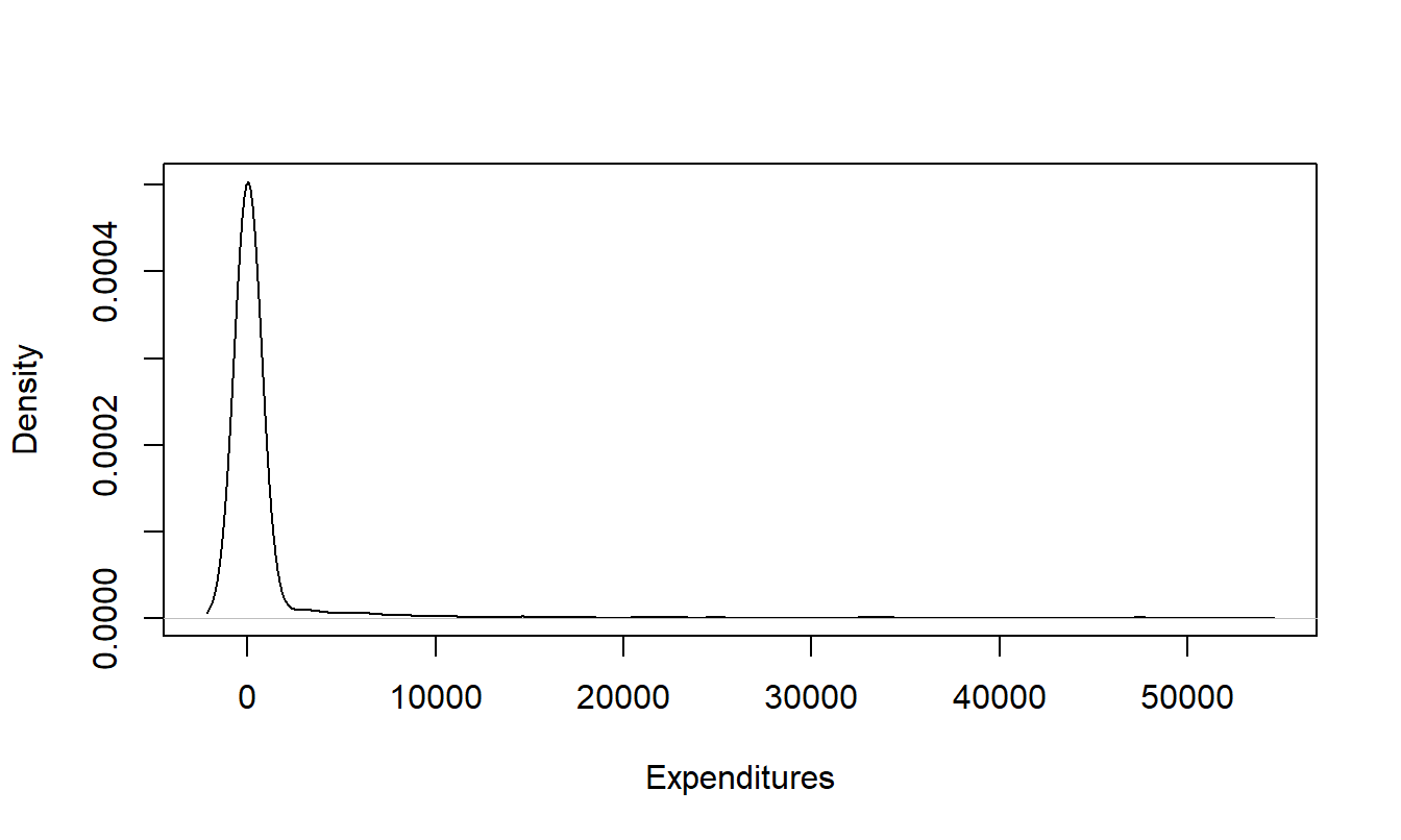
Figure 13.1: Smooth Empirical Histogram of Positive Inpatient Expenditures. The largest expenditure is omitted.
R Code to Produce Figure 13.1
A gamma regression model using a logarithmic link was fit to inpatient expenditures using all explanatory variables. The results of this model fit appear in Table 13.6. Here, we see that many of the potentially important determinants of medical expenditures are not statistically significant. This is common in expenditure analysis, where variables help predict the frequency although are not as useful in explaining severity.
Because of collinearity, we have seen in linear models that having too many variables in a fitted model can lead to statistical insignificance of important variables and even cause signs to be reversed. For a simpler model, we removed the Asian, Native American and the uninsured variables because they account for a small subset of our sample. We also used only the POOR variable for self-reported health status and only POORNEG for income, essentially reducing these categorical variables to binary variables. Table 13.6, under the heading “Reduced Model,” reports the result of this model fit. This model has almost the same goodness of fit statistic, \(AIC\), suggesting that it is a reasonable alternative. Under the reduced model fit, the variables COUNTIP (inpatient count), AGE, COLLEGE and POORNEG, are statistically significant variables. For these significant variables, the signs are intuitively appealing. For example, the positive coefficient associated with COUNTIP means that as the number of inpatient visits increases, the total expenditures increases, as anticipated.
For another alternative model specification, Table 13.6 also shows a fit of an inverse gaussian model with a logarithmic link. From the \(AIC\) statistic, we see that this model does not fit nearly as well as the gamma regression model. All variables are statistically insignificant, making it difficult to interpret this model.
Table 13.6. Comparison of Gamma and Inverse Gaussian Regression Models
\[ \small{ \begin{array}{l|rr|rr|rr} \hline & \text{Gamma} & &\text{Gamma}&&\text{Inverse}&\text{Gaussian} \\ \hline & \text{Full} &\text{Model}& \text{Reduced} & \text{Model}&\text{Reduced}&\text{Model} \\ \hline & \textit{Parameter} & & Parameter & & Parameter & \\ \text{Effect} & Estimate & t\text{-value} & Estimate & t\text{-value} & Estimate & t\text{-value} \\ \hline Intercept & 6.891 & 13.080 & 7.859 & 17.951 & 6.544 & 3.024 \\ COUNTIP & 0.681 & 6.155 & 0.672 & 5.965 & 1.263 & 0.989 \\ AGE & 0.021 & 3.024 & 0.015 & 2.439 & 0.018 & 0.727 \\ GENDER & -0.228 & -1.263 & -0.118 & -0.648 & 0.363 & 0.482 \\ ASIAN & -0.506 & -1.029 & & & & \\ BLACK & -0.331 & -1.656 & -0.258 & -1.287 & -0.321 & -0.577 \\ NATIVE & -1.220 & -2.217 & & & & \\ NORTHEAST & -0.372 & -1.548 & -0.214 & -0.890 & 0.109 & 0.165 \\ MIDWEST & 0.255 & 1.062 & 0.448 & 1.888 & 0.399 & 0.654 \\ SOUTH & 0.010 & 0.047 & 0.108 & 0.516 & 0.164 & 0.319 \\\hline COLLEGE & -0.413 & -1.723 & -0.469 & -2.108 & -0.367 & -0.606 \\ HIGHSCHOOL & -0.155 & -0.827 & -0.210 & -1.138 & -0.039 & -0.078 \\\hline POOR & -0.003 & -0.010 & 0.167 & 0.706 & 0.167 & 0.258 \\ FAIR & -0.194 & -0.641 & & & & \\ GOOD & 0.041 & 0.183 & & & & \\ VGOOD & 0.000 & 0.000 & & & & \\ MNHPOOR & -0.396 & -1.634 & -0.314 & -1.337 & -0.378 & -0.642 \\ ANYLIMIT & 0.010 & 0.053 & 0.052 & 0.266 & 0.218 & 0.287 \\\hline MINCOME & 0.114 & 0.522 & & & & \\ LINCOME & 0.536 & 2.148 & & & & \\ NPOOR & 0.453 & 1.243 & & & & \\ POORNEG & -0.078 & -0.308 & -0.406 & -2.129 & -0.356 & -0.595 \\ INSURE & 0.794 & 3.068 & & & & \\\hline Scale & 1.409 & 9.779 & 1.280 & 9.854 & 0.026 & 17.720 \\ \hline Log-Likelihood & -1,558.67 && -1,567.93 && -1,669.02 \\ AIC & 3,163.34 && 3,163.86 && 3,366.04 \\ \hline \end{array} } \]
R Code to Produce Table 13.6
13.5 Residuals
One way of selecting an appropriate model is to fit a tentative specification and analyze ways of improving it. This diagnostic method relies on residuals. In the linear model, we defined residuals as the response minus the corresponding fitted values. In a GLM context, we refer to these as “raw residuals,” denoted as \(y_i - \widehat{\mu}_i\). As we have seen, residuals are useful for:
- discovering new covariates or the effects of nonlinear patterns in existing covariates,
- identifying poorly fitting observations,
- quantifying the effects of individual observations on model parameters and
- revealing other model patterns, such as heteroscedasticity or time trends.
As this section emphasizes, residuals are also the building blocks for many goodness of fit statistics.
As we saw in Section 11.1 on binary dependent variables, analysis of raw residuals can be meaningless in some nonlinear contexts. Cox and Snell (1968, 1971) introduced a general notion of residuals that is more useful in nonlinear models than the simple raw residuals. For our applications, we assume that \(y_i\) has a distribution function F(\(\cdot\)) that is indexed by explanatory variables \(\mathbf{x}_i\) and a vector of parameters \(\boldsymbol \theta\) denoted as F(\(\mathbf{x}_i,\boldsymbol \theta\)). Here, the distribution function is common to all observations but the distribution varies through the explanatory variables. The vector of parameters \(\boldsymbol \theta\) includes the regression parameters \(\boldsymbol \beta\) as well as scale parameters. With knowledge of F(\(\cdot\)), we now assume that a new function R(\(\cdot\)) can be computed such that \(\varepsilon_i = \mathrm{R}(y_i; \mathbf{x}_i,\boldsymbol \theta)\), where \(\varepsilon_i\) are identically and independently distributed. Here, the function R(\(\cdot\)) depends on explanatory variables \(\mathbf{x}_i\) and parameters \(\boldsymbol \theta\). The Cox-Snell residuals are then \(e_i = \mathrm{R}(y_i; \mathbf{x}_i,\widehat{\boldsymbol \theta})\). If the model is well-specified and the parameter estimates \(\widehat{\boldsymbol \theta}\) are close to the model parameters \(\boldsymbol \theta\), then the residuals \(e_i\) should be close to i.i.d.
To illustrate, in the linear model we use the residual function \(\mathrm{R}(y_i; \mathbf{x}_i,\boldsymbol \theta) = y_i - \mathbf{x}_i^{\prime} \boldsymbol \beta =y_i - \mu_i = \varepsilon_i,\) resulting in (ordinary) raw residuals. Another choice is to rescale by the standard deviation \[ \mathrm{R}(y_i; \mathbf{x}_i,\boldsymbol \theta) = \frac{y_i - \mu_i}{\sqrt{\mathrm{Var~} y_i}} , \] that yields Pearson residuals.
Another type of residual is based on a first transforming the response with a known function h(\(\cdot\)), \[ \mathrm{R}(y_i; \mathbf{x}_i,\boldsymbol \theta) = \frac{\mathrm{h}(y_i) - \mathrm{E~} \mathrm{h}(y_i)}{\sqrt{\mathrm{Var~}\mathrm{h}(y_i)}} . \] Choosing the function so that h(\(y_i\)) is approximately normally distributed yields Anscombe residuals. Another popular choice is to choose the transform so that the variance is stabilized. Table 13.7 gives transforms for the binomial, Poisson and gamma distributions.
Table 13.7. Approximate Normality and Variance-Stabilizing Transforms
\[ \small{ \begin{array}{lcc} \hline \text{Distribution} & \text{Approximate Normality} & \text{Variance-Stabilizing} \\ & \text{Transform} & \text{Transform} \\ \hline \text{Binomial}(m,p) & \frac{\mathrm{h}_B(y/m)-[\mathrm{h}_B(p)+(p(1-p))^{-1/3}(2p-1)/(6m)]}{(p(1-p)^{1/6}/\sqrt{m}} & \frac{\sin^{-1}(\sqrt{y/m})-\sin^{-1}(\sqrt{p})}{a/(2\sqrt{m})} \\ \text{Poisson}(\lambda) & 1.5 \lambda^{-1/6} \left[ y^{2/3}-(\lambda^{2/3}-\lambda^{-1/3}/9) \right] & 2(\sqrt{y}-\sqrt{\lambda})\\ \text{Gamma}(\alpha, \gamma) & 3 \alpha^{1/6} \left[ (y/\gamma)^{1/3}-(\alpha^{1/3}-\alpha^{-2/3}/9) \right] & \text{Not considered}\\ \hline \\ \end{array} } \] Note: \(\mathrm{h}_B(u) = \int_0^u s^{-1/3} (1-s)^{-1/3}ds\) is the incomplete beta function evaluated at \((2/3, 2/3)\), up to a scalar constant. Source: Pierce and Schafer (1986).
Another widely used choice in GLM studies are deviance residuals, defined as \[ \mathrm{sign} \left(y_i - \widehat{\mu}_i \right) \sqrt{2 \left( \ln \mathrm{f}(y_i;\theta_{i,SAT}) - \ln \mathrm{f}(y_i;\widehat{\theta}_{i}) \right)}. \] Section 13.3.3 introduced the parameter estimates of the saturated model, \(\theta_{i,SAT}\). As discussed by Pierce and Schafer (1986), deviance residuals are very close to Anscombe residuals in many cases - we can check deviance residuals for approximate normality. Further, deviance residuals can be defined readily for any GLM model and are easy to compute.
13.6 Tweedie Distribution
We have seen that the natural exponential family includes continuous distributions, such as the normal and gamma, as well as discrete distributions, such as the binomial and Poisson. It also includes distributions that are mixtures of discrete and continuous components. In insurance claims modeling, the most widely used mixture is the Tweedie (1984) distribution. It has a positive mass at zero representing no claims and a continuous component for positive values representing the amount of a claim.
The Tweedie distribution is defined as a Poisson sum of gamma random variables, known as an aggregate loss in actuarial science. Specifically, suppose that \(N\) has a Poisson distribution with mean \(\lambda\), representing the number of claims. Let {\(y_j\)} be an i.i.d. sequence, independent of \(N\), with each \(y_j\) having a gamma distribution with parameters \(\alpha\) and \(\gamma\), representing the amount of a claim. Then, \(S_N = y_1 + \ldots + y_N\) is Poisson sum of gammas. Section 16.5 will discuss aggregate loss models in further detail. This section focuses on the important special case of the Tweedie distribution.
To understand the mixture aspect of the Tweedie distribution, first note that it is straightforward to compute the probability of zero claims as \[ \Pr ( S_N=0) = \Pr (N=0) = e^{-\lambda}. \] The distribution function can be computed using conditional expectations, \[ \Pr ( S_N \le y) = e^{-\lambda}+\sum_{n=1}^{\infty} \Pr(N=n) \Pr(S_n \le y), ~~~~~y \geq 0. \] Because the sum of i.i.d. gammas is a gamma, \(S_n\) (not \(S_N\)) has a gamma distribution with parameters \(n\alpha\) and \(\gamma\). Thus, for \(y>0\), the density of the Tweedie distribution is \[\begin{equation} \mathrm{f}_{S}(y) = \sum_{n=1}^{\infty} e^{-\lambda} \frac{\lambda ^n}{n!} \frac{\gamma^{n \alpha}}{\Gamma(n \alpha)} y^{n \alpha -1} e^{-y \gamma}. \tag{13.9} \end{equation}\]
At first glance, this density does not appear to be a member of the linear exponential family given in equation (13.2). To see the relationship, we first calculate the moments using iterated expectations as \[\begin{equation} \mathrm{E~}S_N = \lambda \frac{\alpha}{\gamma}~~~~~~\mathrm{and}~~~~~ \mathrm{Var~}S_N = \frac{\lambda \alpha}{\gamma^2} (1+\alpha). \tag{13.10} \end{equation}\] Now, define three parameters \(\mu, \phi, p\) through the relations \[ \lambda = \frac{\mu^{2-p}}{\phi (2-p)},~~~~~~\alpha = \frac{2-p}{p-1}~~~~~~\mathrm{and}~~~~~ \frac{1}{\gamma} = \phi(p-1)\mu^{p-1}. \] Inserting these new parameters in equation (13.9) yields \[\begin{equation} \mathrm{f}_{S}(y) = \exp \left[ \frac{-1}{\phi} \left( \frac{\mu^{2-p}}{2-p} + \frac{y}{(p-1)\mu^{p-1}} \right) + S(y,\phi) \right]. \tag{13.11} \end{equation}\] We leave the calculation of \(S(y,\phi)\) as an exercise.
Thus, the Tweedie distribution is a member of the linear exponential family. Easy calculations show that \[\begin{equation} \mathrm{E~}S_N = \mu~~~~~~\mathrm{and}~~~~~ \mathrm{Var~}S_N = \phi \mu^p, \tag{13.12} \end{equation}\] where \(1<p<2.\) Examining our variance function Table 13.1, the Tweedie distribution can also be viewed as a choice that is intermediate between the Poisson and the gamma distributions.
Video: Section Summary
13.7 Further Reading and References
A more extensive treatment of GLM may be found in the classic work by McCullagh and Nelder (1989) or the gentler introduction by Dobson (2002). de Jong and Heller (2008) provide a recent book-long introduction to GLMs with a special insurance emphasis.
GLMs have enjoyed substantial attention from property and casualty (general) insurance practicing actuaries recently, see Anderson et al. (2004) and Clark and Thayer (2004) for introductions.
Mildenhall (1999) provides a systematic analysis of the connection between GLM models and algorithms for assessing different rating plans. Fu and Wu (2008) provide an updated version, introducing a broader class of iterative algorithms that tie nicely to GLM models.
For further information on the Tweedie distribution, see J{}rgensen and de Souza (1994) and Smyth and J{}rgensen (2002).
Chapter References
- Anderson, Duncan, Sholom Feldblum, Claudine Modlin, Doris Schirmacher, Ernesto Schirmacher and Neeza Thandi (2004). A practitioner’s guide to generalized linear models. Casualty Actuarial Society 2004 Discussion Papers 1-116, Casualty Actuarial Society.
- Baxter, L. A., S. M. Coutts and G. A. F. Ross (1980). Applications of linear models in motor insurance. Proceedings of the 21st International Congress of Actuaries. Zurich. pp. 11-29.
- Clark, David R. and Charles A. Thayer (2004). A primer on the exponential family of distributions. Casualty Actuarial Society 2004 Discussion Papers 117-148, Casualty Actuarial Society.
- Cox, David R. and E. J. Snell (1968). A general definition of residuals. Journal of the Royal Statistical Society, Series B, 30, 248-275.
- Cox, David R. and E. J. Snell (1971). On test statistics computed from residuals. Biometrika 71, 589-594.
- Dobson, Annette J. (2002). An Introduction to Generalized Linear Models, Second Edition. Chapman & Hall, London.
- Fu, Luyang and Cheng-sheng Peter Wu (2008). General iteration algorithm for classification ratemaking. Variance 1(2), 193-213, Casualty Actuarial Society.
- de Jong, Piet and Gillian Z. Heller (2008). Generalized Linear Models for Insurance Data. Cambridge University Press, Cambridge, UK.
- J{}rgensen, Bent and Marta C. Paes de Souza (1994). Fitting Tweedie’s compound Poisson model to insurance claims data. Scandinavian Actuarial Journal 1994;1, 69-93.
- McCullagh, P. and J.A. Nelder (1989). Generalized Linear Models, Second Edition. Chapman & Hall, London.
- Mildenhall, Stephen J. (1999). A systematic relationship between minimum bias and generalized linear models. Casualty Actuarial Society Proceedings 86, Casualty Actuarial Society.
- Pierce, Donald A. and Daniel W. Schafer (1986). Residuals in generalized linear models. Journal of the American Statistical Association 81, 977-986.
- Smyth, Gordon K. and Bent J{}rgensen (2002). Fitting Tweedie’s compound Poisson model to insurance claims data: Dispersion modelling. Astin Bulletin 32(1), 143-157.
- Tweedie, M. C. K. (1984). An index which distinguishes between some important exponential families. In Statistics: Applications and New Directions. Proceedings of the Indian Statistical Golden Jubilee International Conference* (Editors J. K. Ghosh and J. Roy), pp. 579-604. Indian Statistical Institute, Calcutta.
13.8 Exercises
13.1 Verify the entries in Table 13.8 for the gamma distribution. Specifically:
Show that the gamma is a member of the linear exponential family of distributions.
Describe the components of the linear exponential family ($ , , b(), S(y,)$) in terms of the parameters of the gamma distribution.
Show that the mean and variance of the gamma and linear exponential family distributions agree.
13.2 Ratemaking Classification. This exercise considers the data described in the Section 13.2.2 ratemaking classification example using data in Table 13.3.
Fit a gamma regression model using a log-link function with claim counts as weights (\(w_i\)). Use the categorical explanatory variables age group and vehicle use to estimate expected average severity.
Based on your estimated parameters in part (a), verify the estimated expected severities in Table 13.4.
13.3 Verify that the Tweedie distribution is a member of the linear exponential family of distributions by checking equation (13.9). In particular, provide an expression for \(S(y,\phi)\) (note that \(S(y,\phi)\) also depends on \(p\) but not on \(\mu\)). You may wish to see Clark and Thayer (2004) to check your work. Further, verify the moments in equation (13.10).
13.9 Technical Supplements - Exponential Family
13.9.1 Linear Exponential Family of Distributions
The distribution of the random variable \(y\) may be discrete, continuous or a mixture. Thus, f(.) in equation (13.2) may be interpreted to be a density or mass function, depending on the application. Table 13.8 provides several examples, including the normal, binomial and Poisson distributions.
Table 13.8. Selected Distributions of the One-Parameter Exponential Family
\[ \scriptsize{ \begin{array}{l|ccccc} \hline & & \text{Density or} & & & \\ \text{Distribution} & \text{Parameters} & \text{Mass Function} & \text{Components} & \mathrm{E}~y & \mathrm{Var}~y \\ \hline \text{General} & \theta,~ \phi & \exp \left( \frac{y\theta -b(\theta )}{\phi } +S\left( y,\phi \right) \right) & \theta,~ \phi, b(\theta), S(y, \phi) & b^{\prime}(\theta) & b^{\prime \prime}(\theta) \phi \\ \text{Normal} & \mu, \sigma^2 & \frac{1}{\sigma \sqrt{2\pi }}\exp \left( - \frac{(y-\mu )^{2}}{2\sigma ^{2}}\right) & \mu, \sigma^2, \frac{\theta^2}{2}, - \left(\frac{y^2}{2\phi} + \frac{\ln(2 \pi \phi)}{2} \right) & \theta=\mu & \phi= \sigma^2 \\ \text{Binomal} & \pi & {n \choose y} \pi ^y (1-\pi)^{n-y} & \ln \left(\frac{\pi}{1-\pi} \right), 1, n \ln(1+e^{\theta} ), & n \frac {e^{\theta}}{1+e^{\theta}} & n \frac {e^{\theta}}{(1+e^{\theta})^2} \\ & & & \ln {n \choose y} & = n \pi & = n \pi (1-\pi) \\ \text{Poisson} & \lambda & \frac{\lambda^y}{y!} \exp(-\lambda) & \ln \lambda, 1, e^{\theta}, - \ln (y!) & e^{\theta} = \lambda & e^{\theta} = \lambda \\ \text{Negative} & r,p & \frac{\Gamma(y+r)}{y! \Gamma(r)} p^r ( 1-p)^y & \ln(1-p), 1, -r \ln(1-e^{\theta}), & \frac{r(1-p)}{p} & \frac{r(1-p)}{p^2} \\ \ \ \ \text{Binomial}^{\ast} & & & ~~~\ln \left[ \frac{\Gamma(y+r)}{y! \Gamma(r)} \right] & = \mu & = \mu+\mu^2/r \\ \text{Gamma} & \alpha, \gamma & \frac{\gamma ^ \alpha}{\Gamma (\alpha)} y^{\alpha -1 }\exp(-y \gamma) & - \frac{\gamma}{\alpha}, \frac{1}{\alpha}, - \ln ( - \theta), -\phi^{-1} \ln \phi & - \frac{1}{\theta} = \frac{\alpha}{\gamma} & \frac{\phi}{\theta ^2} = \frac{\alpha}{\gamma ^2} \\ & & & - \ln \left( \Gamma(\phi ^{-1}) \right) + (\phi^{-1} - 1) \ln y & & \\ \text{Inverse} & \mu, \lambda & \sqrt{\frac{\lambda}{2 \pi y^3} } \exp \left(- \frac{\lambda (y-\mu)^2}{2 \mu^2 y} \right) & -1/( 2\mu^2), 1/\lambda, -\sqrt{-2 \theta}, & \left(-2 \theta \right)^{-1/2} & \phi (-2 \theta)^{-3/2} \\ \ \ \ \text{Gaussian} & & & \theta/(\phi y) - 0.5 \ln (\phi 2 \pi y^3 ) & = \mu & = \frac{\mu^3}{\lambda} \\ \text{Tweedie} & & \textit{See Section 13.6}\\ \hline \\ \end{array} } \] \(^{\ast}\) This assumes that the parameter \(r\) is fixed but need not be an integer.
13.9.2 Moments
To assess the moments of exponential families, it is convenient to work with the moment generating function. For simplicity, we assume that the random variable \(y\) is continuous. Define the moment generating function
\[\begin{eqnarray*} M(s) &=& \mathrm{E}~ e^{sy} = \int \exp \left( sy+ \frac{y \theta - b(\theta)}{\phi} + S(y, \phi) \right) dy \\ &=& \exp \left(\frac{b(\theta + s \phi) - b(\theta)}{\phi} \right) \int \exp \left( \frac{y(\theta + s\phi) - b(\theta+s\phi)}{\phi} + S(y, \phi) \right) dy \\ &=& \exp \left(\frac{b(\theta + s \phi) - b(\theta)}{\phi} \right), \end{eqnarray*}\] because \(\int \exp \left( \frac{1}{\phi} \left[ y(\theta + s\phi) - b(\theta+s\phi) \right] + S(y, \phi) \right) dy=1\). With this expression, we can generate the moments. Thus, for the mean, we have \[\begin{eqnarray*} \mathrm{E}~ y &=& M^{\prime}(0) = \left . \frac{\partial}{\partial s} \exp \left(\frac{b(\theta + s \phi) - b(\theta)}{\phi} \right) \right | _{s=0} \\ &=& \left[ b^{\prime}(\theta + s \phi ) \exp \left( \frac{b(\theta + s \phi) - b(\theta)}{\phi} \right) \right] _{s=0} = b^{\prime}(\theta). \end{eqnarray*}\]
Similarly, for the second moment, we have \[\begin{eqnarray*} M^{\prime \prime}(s) &=& \frac{\partial}{\partial s} \left[ b^{\prime}(\theta + s \phi) \exp \left(\frac{b(\theta + s \phi) - b(\theta)}{\phi} \right) \right] \\ &=& \phi b^{\prime \prime}(\theta + s \phi) \exp \left(\frac{b(\theta + s \phi) - b(\theta)}{\phi} \right) + (b^{\prime}(\theta + s \phi))^2 \left(\frac{b(\theta + s \phi) - b(\theta)}{\phi} \right). \end{eqnarray*}\] This yields \(\mathrm{E}y^2 = M^{\prime \prime}(0)\) \(= \phi b^{\prime \prime}(\theta) + (b^{\prime}(\theta))^2\) and \(\mathrm{Var}~y =\phi b^{\prime \prime}(\theta)\).
13.9.3 Maximum Likelihood Estimation for General Links
For general links, we no longer assume the relationship \(\theta_i=\mathbf{x}_i^{\mathbf{\prime }}\boldsymbol \beta\) but assume that \(\boldsymbol \beta\) is related to \(\theta_i\) through the relations \(\mu _i=b^{\prime }(\theta_i)\) and \(\mathbf{x}_i^{\mathbf{\prime }}\boldsymbol \beta = g\left( \mu _i\right)\). We continue to assume that the scale parameter varies by observation so that \(\phi_i = \phi/w_i\), where \(w_i\) is a known weight function. Using equation (13.4), we have that the \(j\)th element of the score function is \[ \frac{\partial }{\partial \beta _{j}}\ln \mathrm{f}\left( \mathbf{y}\right) =\sum_{i=1}^n \frac{\partial \theta_i}{\partial \beta _{j}} \frac{y_i-\mu _i}{\phi _i} , \] because \(b^{\prime }(\theta_i)=\mu _i\). Now, use the chain rule and the relation \(\mathrm{Var~}y_i=\phi _ib^{\prime \prime }(\theta_i)\) to get \[ \frac{\partial \mu _i}{\partial \beta _{j}}=\frac{\partial b^{\prime }(\theta_i)}{\partial \beta _{j}}=b^{\prime \prime }(\theta_i)\frac{ \partial \theta_i}{\partial \beta _{j}}=\frac{\mathrm{Var~}y_i}{\phi _i}\frac{\partial \theta_i}{\partial \beta _{j}}. \] Thus, we have \[ \frac{\partial \theta_i}{\partial \beta _{j}}\frac{1}{\phi _i}=\frac{ \partial \mu _i}{\partial \beta _{j}}\frac{1}{\mathrm{Var~}y_i}. \] This yields \[ \frac{\partial }{\partial \beta _{j}}\ln \mathrm{f}\left( \mathbf{y}\right) =\sum_{i=1}^n \frac{\partial \mu _i}{\partial \beta _{j}}\left( \mathrm{Var~}y_i\right) ^{-1}\left( y_i-\mu _i\right) , \] that we summarize as \[\begin{equation} \frac{\partial L(\boldsymbol \beta) }{\partial \boldsymbol \beta } = \frac{\partial }{\partial \boldsymbol \beta }\ln \mathrm{f}\left( \mathbf{y}\right) =\sum_{i=1}^n \frac{\partial \mu _i}{\partial \boldsymbol \beta}\left( \mathrm{Var~}y_i\right) ^{-1}\left( y_i-\mu _i\right) , \tag{13.13} \end{equation}\] which is known as the generalized estimating equations form.
Solving for roots of the score equation \(L(\boldsymbol \beta) = \mathbf{0}\) yield maximum likelihood estimates, \(\mathbf{b}_{MLE}\). In general, this requires iterative numerical methods. An exception is the following special case.
Special Case. No Covariates. Suppose that \(k=1\) and that \(x_i =1\). Thus, \(\beta = \eta = g(\mu),\) and \(\mu\) does not depend on \(i\). Then, from the relation \(\mathrm{Var~}y_i = \phi b^{\prime \prime}(\theta)/w_i\) and equation (13.13), the score function is \[ \frac{\partial L( \beta) }{\partial \beta } = \frac{\partial \mu}{\partial \beta} ~ \frac{1}{\phi b^{\prime \prime}(\theta)} \sum_{i=1}^n w_i \left( y_i-\mu \right) . \] Setting this equal zero yields \(\overline{y}_w = \sum_i w_i y_i / \sum_i w_i = \widehat{\mu}_{MLE} = g^{-1}(b_{MLE})\), or \(b_{MLE}=g(\overline{y}_w),\) where \(\overline{y}_w\) is a weighted average of \(y\)’s.
For the information matrix, use the independence among subjects and equation (13.13) to get \[\begin{eqnarray} \mathbf{I}(\boldsymbol \beta) &=& \mathrm{E~} \left( \frac{\partial L(\boldsymbol \beta) }{\partial \boldsymbol \beta } \frac{\partial L(\boldsymbol \beta) }{\partial \boldsymbol \beta ^{\prime}} \right) \nonumber \\ &=& \sum_{i=1}^n \frac{\partial \mu _i}{\partial \boldsymbol \beta}~\mathrm{E} \left( \left( \mathrm{Var~}y_i\right) ^{-1}\left( y_i-\mu _i\right)^2 \left( \mathrm{Var~}y_i\right) ^{-1}\right) \frac{\partial \mu _i}{\partial \boldsymbol \beta ^{\prime}} \nonumber \\ &=& \sum_{i=1}^n \frac{\partial \mu _i}{\partial \boldsymbol \beta} \left( \mathrm{Var~}y_i\right) ^{-1} \frac{\partial \mu _i}{\partial \boldsymbol \beta ^{\prime}} . \tag{13.14} \end{eqnarray}\]
Taking the square root of the diagonal elements of the inverse of \(\mathbf{I}(\boldsymbol \beta)\), after inserting parameter estimates in the mean and variance functions, yields model-based standard errors. For data where the correct specification of the variance component is in doubt, one replaces Var \(y_i\) by an unbiased estimate \((y_i - \mu_i)^2\). The resulting estimator \[ se(b_j) = \sqrt{ jth~diagonal~element~of~ [\sum_{i=1}^n \frac{\partial \mu _i}{\partial \boldsymbol \beta} (y_i - \mu_i)^{-2} \frac{\partial \mu _i}{\partial \boldsymbol \beta ^{\prime}} ]|_{\boldsymbol \beta = \mathbf{b}_{MLE}}^{-1}} \]
is known as the empirical, or robust, standard error.
13.9.4 Iterated Reweighted Least Squares
To see how general iterative methods work, we use the canonical link so that \(\eta_i = \theta_i\). Then, the score function is given in equation (13.6) and the Hessian is in equation (13.8). Using the Newton-Raphson equation (11.15) in Section 11.9 yields \[\begin{equation} \boldsymbol \beta_{NEW} = \boldsymbol \beta_{OLD} - \left( \sum_{i=1}^n w_i b^{\prime \prime}(\mathbf{x}_i^{\prime} \boldsymbol \beta _{OLD}) \mathbf{x}_i \mathbf{x}_i^{\prime} \right)^{-1} \left( \sum_{i=1}^n w_i (y_i - b^{\prime}(\mathbf{x}_i^{\prime} \boldsymbol \beta_{OLD})) \mathbf{x}_i \right) . \tag{13.15} \end{equation}\] Note that because the matrix of second derivatives is non-stochastic, the Newton-Raphson is equivalent to the Fisher scoring algorithm. As described in Section 13.3.1, the estimation of \(\boldsymbol \beta\) does not require knowledge of \(\phi\).
Continue using the canonical link and define an “adjusted dependent variable” \[ y_i^{\ast}(\boldsymbol \beta) = \mathbf{x}_i^{\prime} \boldsymbol \beta + \frac{y_i - b^{\prime}(\mathbf{x}_i^{\prime} \boldsymbol \beta)}{b^{\prime \prime}(\mathbf{x}_i^{\prime} \boldsymbol \beta)}. \] This has variance \[ \mathrm{Var~}y_i^{\ast}(\boldsymbol \beta) = \frac{\mathrm{Var~}y_i}{(b^{\prime \prime}(\mathbf{x}_i^{\prime} \boldsymbol \beta))^2} = \frac{\phi_i b^{\prime \prime}(\mathbf{x}_i^{\prime} \boldsymbol \beta)}{(b^{\prime \prime}(\mathbf{x}_i^{\prime} \boldsymbol \beta))^2} = \frac{\phi/ w_i }{b^{\prime \prime}(\mathbf{x}_i^{\prime} \boldsymbol \beta)}. \] Use the new weight as the reciprocal of the variance, \(w_i(\boldsymbol \beta)=w_i b^{\prime \prime}(\mathbf{x}_i^{\prime} \boldsymbol \beta) / \phi.\) Then, with the expression \[ w_i \left(y_i - b^{\prime}(\mathbf{x}_i^{\prime} \boldsymbol \beta)\right) = w_i b^{\prime \prime}(\mathbf{x}_i^{\prime} \boldsymbol \beta) (y_i^{\ast}(\boldsymbol \beta) - \mathbf{x}_i^{\prime} \boldsymbol \beta) = \phi w_i(\boldsymbol \beta) (y_i^{\ast}(\boldsymbol \beta) - \mathbf{x}_i^{\prime} \boldsymbol \beta), \] from the Newton-Raphson iteration in equation (13.15), we have
\(\boldsymbol \beta_{NEW}\) \[\begin{eqnarray*} ~ &=& \boldsymbol \beta_{OLD} - \left( \sum_{i=1}^n w_i b^{\prime \prime}(\mathbf{x}_i^{\prime} \boldsymbol \beta _{OLD}) \mathbf{x}_i \mathbf{x}_i^{\prime} \right)^{-1} \left( \sum_{i=1}^n w_i (y_i - b^{\prime}(\mathbf{x}_i^{\prime} \boldsymbol \beta_{OLD})) \mathbf{x}_i \right) \\ &=& \boldsymbol \beta_{OLD} - \left( \sum_{i=1}^n \phi w_i(\boldsymbol \beta _{OLD}) \mathbf{x}_i \mathbf{x}_i^{\prime} \right)^{-1} \left( \sum_{i=1}^n \phi w_i(\boldsymbol \beta _{OLD}) (y_i^{\ast}(\boldsymbol \beta_{OLD}) - \mathbf{x}_i^{\prime} \boldsymbol \beta_{OLD})\mathbf{x}_i \right) \\ &=& \boldsymbol \beta_{OLD} - \left( \sum_{i=1}^n w_i(\boldsymbol \beta _{OLD}) \mathbf{x}_i \mathbf{x}_i^{\prime} \right)^{-1} \left( \sum_{i=1}^n w_i(\boldsymbol \beta _{OLD})\mathbf{x}_i y_i^{\ast}(\boldsymbol \beta_{OLD}) - \sum_{i=1}^n w_i(\boldsymbol \beta _{OLD})\mathbf{x}_i \mathbf{x}_i^{\prime} \boldsymbol \beta_{OLD}) \right) \\ &=& \left( \sum_{i=1}^n w_i(\boldsymbol \beta _{OLD}) \mathbf{x}_i \mathbf{x}_i^{\prime} \right)^{-1} \left( \sum_{i=1}^n w_i(\boldsymbol \beta _{OLD})\mathbf{x}_i y_i^{\ast}(\boldsymbol \beta_{OLD}) \right). \end{eqnarray*}\] Thus, this provides a method for iteration using weighted least squares. Iterative reweighted least squares is also available for general links using Fisher scoring, see McCullagh and Nelder (1989) for further details.