Chapter 2 Basic Linear Regression
Chapter Preview. This chapter considers regression in the case of only one explanatory variable. Despite this seeming simplicity, most of the deep ideas of regression can be developed in this framework. By limiting ourselves to the one variable case, we are able to express many calculations using simple algebra. This will allow us to develop our intuition about regression techniques by reinforcing it with simple demonstrations. Further, we can illustrate the relationships between two variables graphically because we are working in only two dimensions. Graphical tools prove to be important for developing a link between the data and a model.
2.1 Correlations and Least Squares
Regression is about relationships. Specifically, we will study how two variables, an \(x\) and a \(y\), are related. We want to be able to answer questions such as, if we change the level of \(x\), what will happen to the level of \(y\)? If we compare two “subjects” that appear similar except for the \(x\) measurement, how will their \(y\) measurements differ? Understanding relationships among variables is critical for quantitative management, particularly in actuarial science where uncertainty is so prevalent.
It is helpful to work with a specific example to become familiar with key concepts. Analysis of lottery sales has not been part of traditional actuarial practice but it is a growth area in which actuaries could contribute.
Example: Wisconsin Lottery Sales. State of Wisconsin lottery administrators are interested in assessing factors that affect lottery sales. Sales consists of online lottery tickets that are sold by selected retail establishments in Wisconsin. These tickets are generally priced at $1.00, so the number of tickets sold equals the lottery revenue. We analyze average lottery sales (SALES) over a forty-week period, April, 1998 through January, 1999, from fifty randomly selected areas identified by postal (ZIP) code within the state of Wisconsin.
Although many economic and demographic variables might influence sales, our first analysis focuses on population (POP) as a key determinant. Chapter 3 will show how to consider additional explanatory variables. Intuitively, it seems clear that geographic areas with more people will have higher sales. So, other things being equal, a larger \(x=POP\) means a larger \(y=SALES.\) However, the lottery is an important source of revenue for the state and we want to be as precise as possible.
A little additional notation will be useful subsequently. In this sample, there are fifty geographic areas and we use subscripts to identify each area. For example, \(y_1\) = 1,285.4 represents sales for the first area in the sample that has population \(x_1\) = 435. Call the ordered pair (\(x_1\), \(y_1\)) = (435, 1285.4) the first observation. Extending this notation, the entire sample containing fifty observations may be represented by (\(x_1\), \(y_1\)), …, (\(x_{50}\), \(y_{50}\)). The ellipses ( … ) mean that the pattern is continued until the final object is encountered. We will often speak of a generic member of the sample, referring to (\(x_i\), \(y_i\)) as the \(i\)th observation.
Data sets can get complicated, so it will help if you begin by working with each variable separately. The two panels in Figure 2.1 show histograms that give a quick visual impression of the distribution of each variable in isolation of the other. Table 2.1 provides corresponding numerical summaries. To illustrate, for the population variable (POP), we see that the area with the smallest number contained 280 people whereas the largest contained 39,098. The average, over 50 ZIP codes, was 9,311.04. For our second variable, sales were as low as 189 and as high as 33,181.
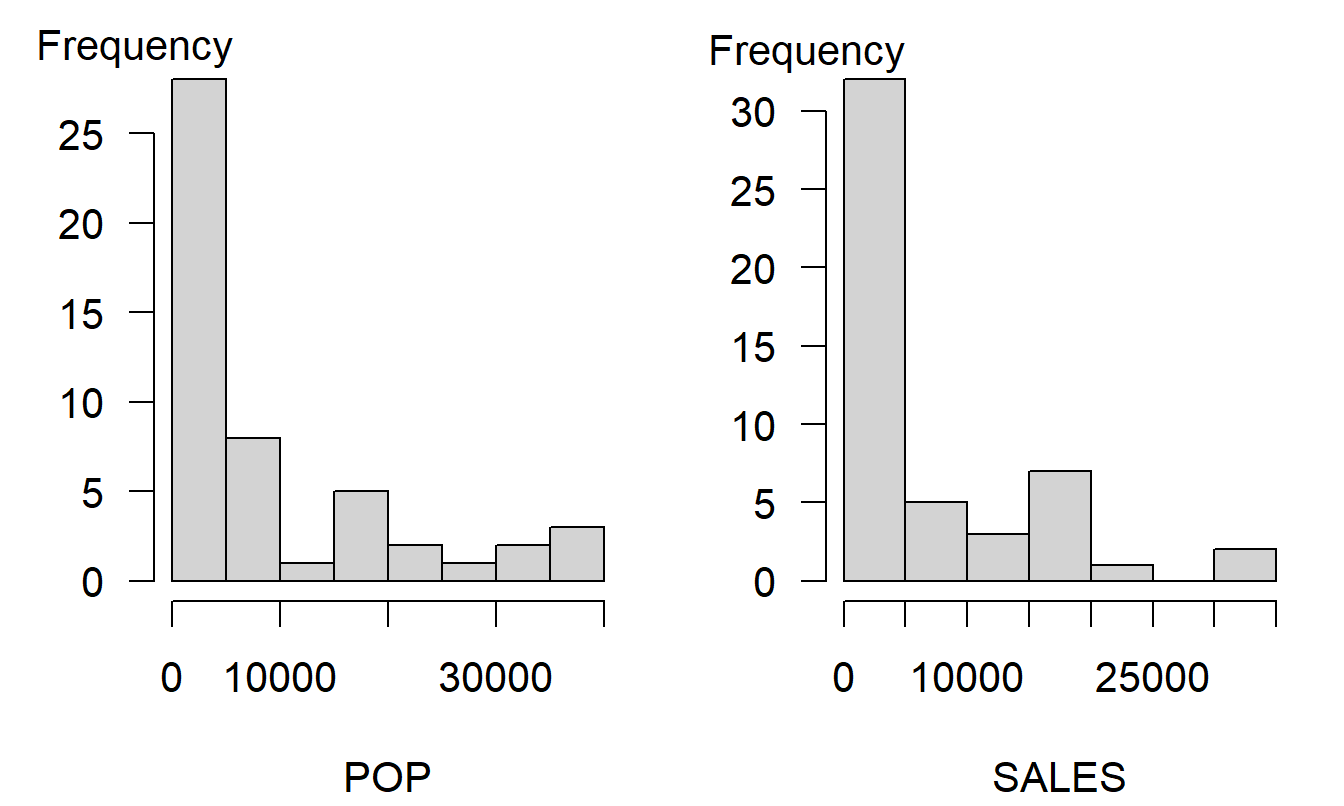
Figure 2.1: Histograms of Population and Sales. Each distribution is skewed to the right, indicating that there are many small areas compared to a few areas with larger sales and populations.
| Mean | Median | Standard Deviation | Minimum | Maximum | |
|---|---|---|---|---|---|
| POP | 9,311 | 4,406 | 11,098 | 280 | 39,098 |
| SALES | 6,495 | 2,426 | 8,103 | 189 | 33,181 |
| Source: Frees and Miller (2003) |
R Code to Produce Figure 2.1 and Table 2.1
As Table 2.1 shows, the basic summary statistics give useful ideas of the structure of key features of the data. After we understand the information in each variable in isolation of the other, we can begin exploring the relationship between the two variables.
Scatter Plot and Correlation Coefficients - Basic Summary Tools
The basic graphical tool used to investigate the relationship between the two variables is a scatter plot such as in Figure 2.2. Although we may lose the exact values of the observations when graphing data, we gain a visual impression of the relationship between population and sales. From Figure 2.2 we see that areas with larger populations tend to purchase more lottery tickets. How strong is this relationship? Can knowledge of the area’s population help us anticipate the revenue from lottery sales? We explore these two questions below.
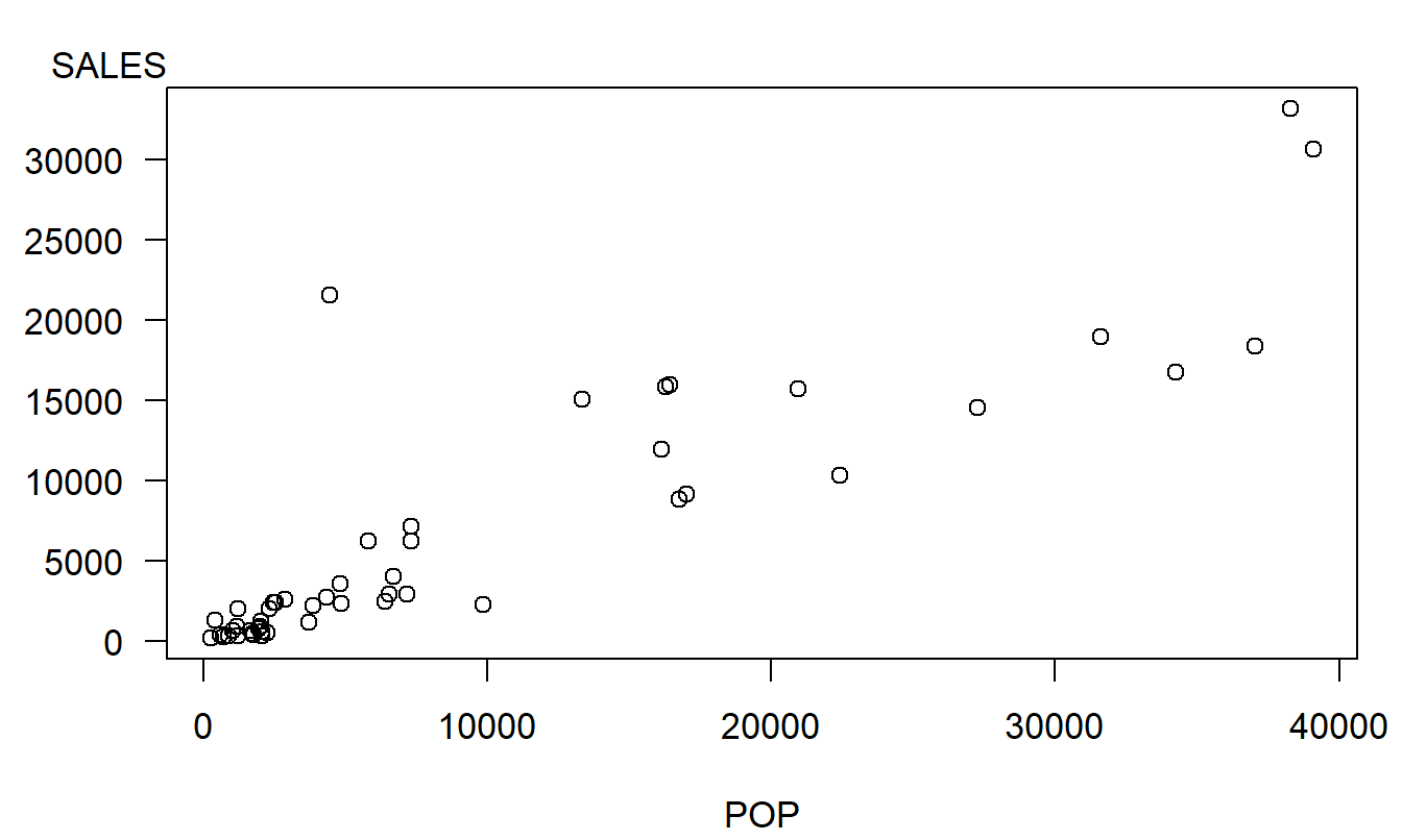
Figure 2.2: A scatter plot of the lottery data. Each of the 50 plotting symbols corresponds to a zip code in the study. This figure suggests that postal areas with larger populations have larger lottery revenues.
R Code to Produce Figure 2.2
One way to summarize the strength of the relationship between two variables is through a correlation statistic.
Definition. The ordinary, or Pearson, correlation coefficient is defined as \[ r=\frac{1}{(n-1)s_xs_y}\sum_{i=1}^{n}\left( x_{i}-\overline{x}\right) \left( y_{i}-\overline{y}\right) . \]
Here, we use the sample standard deviation \(s_y = \sqrt{(n-1)^{-1} \sum_{i=1}^{n}\left( y_i - \overline{y}\right)^{2}}\) defined in Section 1.2, with similar notation for \(s_x\).
Although there are other correlation statistics, the correlation coefficient devised by Pearson (1895) has several desirable properties. One important property is that, for any data set, \(r\) is bounded by -1 and 1, that is, \(-1\leq r\leq 1\). (Exercise 2.3 provides steps for you to check this property.) If \(r\) is greater than zero, the variables are said to be (positively) correlated. If \(r\) is less than zero, the variables are said to be negatively correlated. The larger the coefficient is in absolute value, the stronger is the relationship. In fact, if \(r=1\), then the variables are perfectly correlated. In this case, all of the data lie on a straight line that goes through the lower left and upper right-hand quadrants. If \(r=-1\), then all of the data lie on a line that goes through the upper left and lower right-hand quadrants. The coefficient \(r\) is a measure of a linear relationship between two variables.
The correlation coefficient is said to be location and scale invariant. Thus, each variable’s center of location does not matter in the calculation of \(r\). For example, if we add $100 to the sales of each zip code, each \(y_i\) will increase by 100. However, \(\overline{y}\), the average purchase price will also increase by 100 so that the deviation \(y_i - \overline{y}\) remains unchanged, or invariant. Further, the scale of each variable does not matter in the calculation of \(r\). For example, suppose we divide each population by 1000 so that \(x_i\) now represents population in thousands. Thus, \(\overline{x}\) is also divided by 1000 and you should check that \(s_x\) is also divided by 1000. Thus, the standardized version of \(x_i\), \(\left( x_i-\overline{x}\right) /s_x\), remains unchanged, or invariant. Many statistical packages compute a standardized version of a variable by subtracting the average and dividing by the standard deviation. Now, let’s use \(y_{i,std}=\left( y_i- \overline{y}\right) /s_y\) and \(x_{i,std}=\left( x_i-\overline{x} \right) /s_x\) to be the standardized versions of \(y_i\) and \(x_i\), respectively. With this notation, we can express the correlation coefficient as \(r=(n-1)^{-1}\sum_{i=1}^{n}x_{i,std}\times y_{i,std}.\)
The correlation coefficient is said to be a dimensionless measure. This is because we have taken away dollars, and all other units of measures, by considering the standardized variables \(x_{i,std}\) and \(y_{i,std}\). Because the correlation coefficient does not depend on units of measure, it is a statistic that can readily be compared across different data sets.
In the world of business, the term “correlation” is often used as synonymous with the term “relationship.” For the purposes of this text, we use the term correlation when referring only to linear relationships. The classic nonlinear relationship is \(y=x^{2}\), a quadratic relationship. Consider this relationship and the fictitious data set for \(x\), \(\{-2,1,0,1,2\}\). Now, as an exercise (2.2), produce a rough graph of the data set:
\[ \begin{array}{l|rrrrr} \hline i & 1 & 2 & 3 & 4 & 5 \\ \hline x_i & -2 & -1 & 0 & 1 & 2 \\ y_i & 4 & 1 & 0 & 1 & 4 \\ \hline \end{array} \]
The correlation coefficient for this data set turns out to be \(r=0\) (check this). Thus, despite the fact that there is a perfect relationship between \(x\) and \(y\) (\(=x^{2}\)), there is a zero correlation. Recall that location and scale changes are not relevant in correlation discussions, so we could easily change the values of \(x\) and \(y\) to be more representative of a business data set.
How strong is the relationship between \(y\) and \(x\) for the lottery data? Graphically, the response is a scatter plot, as in Figure 2.2. Numerically, the main response is the correlation coefficient which turns out to be \(r\) = 0.886 for this data set. We interpret this statistic by saying that SALES and POP are (positively) correlated. The strength of the relationship is strong because \(r\) = 0.886 is close to one. In summary, we may describe this relationship by saying that there is a strong correlation between SALES and POP.
Method of Least Squares
Now we begin to explore the question, “Can knowledge of population help us understand sales?” To respond to this question, we identify sales as the response, or dependent, variable. The population variable, which is used to help understand sales, is called the explanatory, or independent, variable.
Suppose that we have available the sample data of fifty sales \(\{y_1, \ldots, y_{50} \}\) and your job is to predict the sales of a randomly selected ZIP code. Without knowledge of the population variable, a sensible predictor is simply \(\overline{y}=6,495\), the average of the available sample. Naturally, you anticipate that areas with larger populations will have larger sales. That is, if you also have knowledge of population, then can this estimate be improved? If so, then by how much?
To answer these questions, the first step assumes an approximate linear relationship between \(x\) and \(y\). To fit a line to our data set, we use the method of least squares. We need a general technique so that, if different analysts agree on the data and agree on the fitting technique, then they will agree on the line. If different analysts fit a data set using eyeball approximations, in general they will arrive at different lines, even using the same data set.
The method begins with the line \(y=b_0^{\ast}+b_1^{\ast}x\), where the intercept and slope, \(b_0^{\ast}\) and \(b_1^{\ast}\), are merely generic values. For the \(i\)th observation, \(y_i-\left( b_0^{\ast}+b_1^{\ast}x_i\right)\) represents the deviation of the observed value \(y_i\) from the line at \(x_i\). The quantity \[ SS(b_0^{\ast},b_1^{\ast})=\sum_{i=1}^{n}\left( y_i-\left( b_0^{\ast}+b_1^{\ast}x_i\right) \right) ^{2} \] represents the sum of squared deviations for this candidate line. The least squares method consists of determining the values of \(b_0^{\ast}\) and \(b_1^{\ast}\) that minimize \(SS(b_0^{\ast},b_1^{\ast})\). This is an easy problem that can be solved by calculus, as follows. Taking partial derivatives with respect to each argument yields \[ \frac{\partial }{\partial b_0^{\ast}}SS(b_0^{\ast},b_1^{\ast})=\sum_{i=1}^{n}(-2)\left( y_i-\left( b_0^{\ast}+b_1^{\ast}x_i\right) \right) \] and \[ \frac{\partial }{\partial b_1^{\ast}}SS(b_0^{\ast},b_1^{\ast})=\sum_{i=1}^{n}(-2x_i)\left( y_i-\left( b_0^{\ast}+b_1^{\ast}x_i\right) \right) . \] The reader is invited to take second partial derivatives to ensure that we are minimizing, not maximizing, this function. Setting these quantities equal to zero and canceling constant terms yields \[ \sum_{i=1}^{n}\left( y_i-\left( b_0^{\ast}+b_1^{\ast}x_i\right) \right) =0 \] and \[ \sum_{i=1}^{n}x_i\left( y_i-\left( b_0^{\ast}+b_1^{\ast}x_i\right) \right) =0, \] which are known as the normal equations. Solving these equations yields the values of \(b_0^{\ast}\) and \(b_1^{\ast}\) that minimize the sum of squares, as follows.
Definition. The least squares intercept and slope estimates are
\[ b_1=r\frac{s_y}{s_x}~~~~~\mathrm{and}~~~~~b_0=\overline{y}-b_1 \overline{x}. \] The line that they determine, \(\widehat{y}=b_0+b_1x\), is called the fitted regression line.
We have dropped the asterisk, or star, notation because \(b_0\) and \(b_1\) are no longer “candidate” values.
Does this procedure yield a sensible line for our Wisconsin lottery sales? Earlier, we computed \(r=0.886\). From this and the basic summary statistics in Table 2.1, we have \(b_1 = 0.886 \left( 8,103\right) /11,098=0.647\) and \(b_0 = 6,495-(0.647)9,311 = 469.7.\) This yields the fitted regression line \[ \widehat{y} = 469.7 + (0.647)x. \] The carat, or “hat,” on top of the \(y\) reminds us that this \(\widehat{y}\), or \(\widehat{SALES}\), is a fitted value. One application of the regression line is to estimate sales for a specific population say, \(x=10,000\). The estimate is the height of the regression line, which is \(469.7 + (0.647)(10,000) = 6,939.7\).
Example: Summarizing Simulations. Regression analysis is a tool for summarizing complex data. In practical work, actuaries often simulate complicated financial scenarios; it is often overlooked that regression can be used to summarize relationships of interest.
To illustrate, Manistre and Hancock (2005) simulated many realizations of a 10-year European put option and demonstrated the relationship between two actuarial risk measures, the value-at-risk (VaR) and the conditional tail expectation (CTE). For one example, these authors examined lognormally distributed stock returns with an initial stock price of $100, so that in 10 years the price of the stock would be distributed as \[ S(Z)=100 \exp \left( (.08) 10 + .15 \sqrt{10} Z \right), \] based on an annual mean return of 8%, standard deviation 15% and the outcome from a standard normal random variable \(Z\). The put option pays the difference between the strike price, that will be taken to be 110 for this example, and \(S(Z)\). The present value of this option is \[ C(Z)= \mathrm{e}^{-0.06(10)} \mathrm{max} \left(0, 110-S(Z) \right), \] based on a 6% discount rate.
To estimate the VaR and CTE, for each \(i\), 1000 i.i.d. standard normal random variables were simulated and used to calculate 1000 present values, \(C_{i1}, \ldots, C_{i,1000}.\) The 95th percentile of these present values is the estimate of the value at risk, denoted as \(VaR_i.\) The average of the highest 50 (\(= (1-.05) \times 1000\)) of the present values is the estimate of the conditional tail expectation, denoted as \(CTE_i\). Manistre and Hancock (2005) performed this calculation \(i=1, \ldots, 1000\) times; the result is presented in Figure 2.3. The scatterplot shows a strong but not perfect relationship between the \(VaR\) and the \(CTE\), the correlation coefficient turns out to be \(r=0.782\).
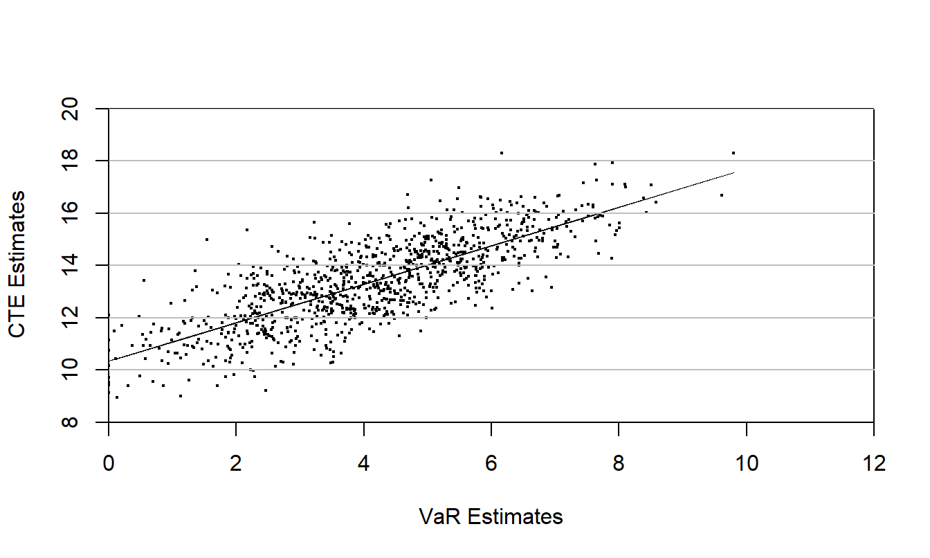
Figure 2.3: Plot of Conditional Tail Expectation (CTE) versus Value at Risk (VaR). Based on \(n=1,000\) simulations from a 10-year European put bond. Source: Manistre and Hancock (2005).
R Code to Produce Figure 2.3
Video: Section Summary
2.2 Basic Linear Regression Model
The scatter plot, correlation coefficient and the fitted regression line are useful devices for summarizing the relationship between two variables for a specific data set. To infer general relationships, we need models to represent outcomes of broad populations.
This chapter focuses on a “basic linear regression” model. The “linear regression” part comes from the fact that we fit a line to the data. The “basic” part is because we use only one explanatory variable, \(x\). This model is also known as a “simple” linear regression. This text avoids this language because it gives the false impression that regression ideas and interpretations with one explanatory variable are always straightforward.
We now introduce two sets of assumptions of the basic model, the “observables” and the “error” representations. They are equivalent but each will help us as we later extend regression models beyond the basics.
\[ {\small \begin{array}{l} \hline \hline &\textbf{Basic Linear Regression Model} \\ &\textbf{Observables Representation Sampling Assumptions} \\ \hline \text{F1}. & \mathrm{E}~y_i=\beta_0 + \beta_1 x_i . \\ \text{F2}. & \{x_1,\ldots ,x_n\} \text{ are non-stochastic variables}. \\ \text{F3}. & \mathrm{Var}~y_i=\sigma ^{2}. \\ \text{F4}. & \{ y_i\} \text{ are independent random variables}. \\ \hline\ \end{array} } \]
The “observables representation” focuses on variables that we can see (or observe), \((x_i,y_i)\). Inference about the distribution of \(y\) is conditional on the observed explanatory variables, so that we may treat \(\{x_1,\ldots ,x_n\}\) as non-stochastic variables (assumption F2). When considering types of sampling mechanisms for \((x_i,y_i)\), it is convenient to think of a stratified random sampling scheme, where values of \(\{x_1,\ldots ,x_n\}\) are treated as the strata, or group. Under stratified sampling, for each unique value of \(x_i\), we draw a random sample from a population. To illustrate, suppose you are drawing from a database of firms to understand stock return performance (\(y\)) and wish to stratify based on the size of the firm. If the amount of assets is a continuous variable, then we can imagine drawing a sample of size 1 for each firm. In this way, we hypothesize a distribution of stock returns conditional on firm asset size.
Digression: You will often see reports that summarize results for the “top 50 managers” or the “best 100 universities,” measured by some outcome variable. In regression applications, make sure that you do not select observations based on a dependent variable, such as the highest stock return, because this is stratifying based on the \(y\), not the \(x\). Chapter 6 will discuss sampling procedures in greater detail.
Stratified sampling also provides motivation for assumption F4, the independence among responses. One can motivate assumption F1 by thinking of \((x_i,y_i)\) as a draw from a population, where the mean of the conditional distribution of \(y_i\) given {\(x_i\)} is linear in the explanatory variable. Assumption F3 is known as homoscedasticity that we will discuss extensively in Section 5.7. See Goldberger (1991) for additional background on this representation.
A fifth assumption that is often implicitly used is:
\[ \text{F}5. ~~\{y_i\}~ \text{ are normally distributed}. \]
This assumption is not required for many statistical inference procedures because central limit theorems provide approximate normality for many statistics of interest. However, formal justification for some, such as \(t\)-statistics, do require this additional assumption.
In contrast to the observables representation, an alternative set of assumptions focuses on the deviations, or “errors,” in the regression, defined as \(\varepsilon_i=y_i-\left( \beta_0 + \beta_1 x_i \right)\).
\[ {\small \begin{array}{l} \hline \hline &\textbf{Basic Linear Regression Model} \\ &\textbf{Error Representation Sampling Assumptions} \\ \hline \text{E1}. & y_i=\beta_0 + \beta_1 x_i + \varepsilon_i . \\ \text{E2}. & \{x_1,\ldots ,x_n\} \text{ are non-stochastic variables}. \\ \text{E3}. & \mathrm{E}~\varepsilon_i=0 \text{ and } \mathrm{Var}~\varepsilon_i=\sigma ^{2}. \\ \text{E4}. & \{ \varepsilon_i\} \text{ are independent random variables}. \\ \hline\ \end{array} } \]
The “error representation” is based on the Gaussian theory of errors (see Stigler, 1986, for a historical background). Assumption E1 assumes that \(y\) is in part due to a linear function of the observed explanatory variable, \(x\). Other unobserved variables that influence the measurement of \(y\) are interpreted to be included in the “error” term \(\varepsilon_i\), which is also known as the “disturbance” term. The independence of errors, E4, can be motivated by assuming that {\(\varepsilon_i\)} are realized through a simple random sample from an unknown population of errors.
Assumptions E1-E4 are equivalent to F1-F4. The error representation provides a useful springboard for motivating goodness of fit measures (Section 2.3). However, a drawback of the error representation is that it draws the attention from the observable quantities \((x_i,y_i)\) to an unobservable quantity, {\(\varepsilon_i\)}. To illustrate, the sampling basis, viewing {\(\varepsilon_i\)} as a simple random sample, is not directly verifiable because one cannot directly observe the sample {\(\varepsilon_i\)}. Moreover, the assumption of additive errors in E1 will be troublesome when we consider nonlinear regression models.
Figure 2.4 illustrates some of the assumptions of the basic linear regression model. The data (\(x_1,y_1\)), (\(x_2,y_2\)) and (\(x_3,y_3\)) are observed and are represented by the circular opaque plotting symbols. According to the model, these observations should be close to the regression line \(\mathrm{E}~y = \beta_0 + \beta_1 x\). Each deviation from the line is random. We will often assume that the distribution of deviations may be represented by a normal curve, as in Figure 2.4.
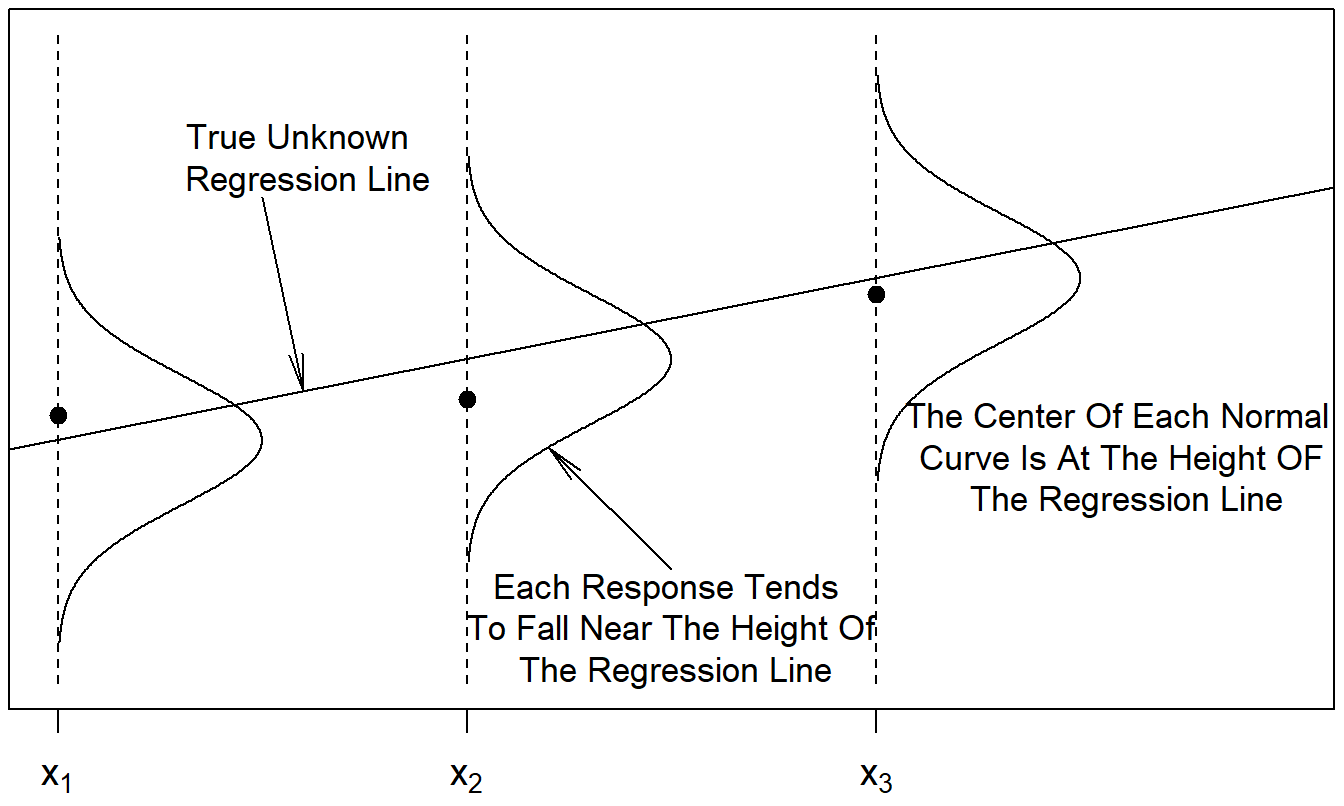
Figure 2.4: The distribution of the response varies by the level of the explanatory variable.
The basic linear regression model assumptions describe the underlying population. Table 2.2 highlights the idea that characteristics of this population can be summarized by the parameters \(\beta_0\), \(\beta_1\) and \(\sigma ^{2}\). In Section 2.1, we summarized data from a sample, introducing the statistics \(b_0\) and \(b_1\). Section 2.3 will introduce \(s^{2}\), the statistic corresponding to the parameter \(\sigma ^{2}\).
Table 2.2. Summary Measures of the Population and Sample
\[ {\small \begin{array}{llccc}\hline\hline & \text{Summary} \\ \text{Data} & \text{Measures} & \text{Intercept} & \text{Slope} & \text{Variance} \\\hline \text{Population} & \text{Parameters} & \beta_0 & \beta_1 & \sigma^2 \\ \text{sample} & \text{Statistics} & b_0 & b_1 & s^2 \\ \hline \end{array} } \]
Video: Section Summary
2.3 Is the Model Useful? Some Basic Summary Measures
Although statistics is the science of summarizing data, it is also the art of arguing with data. This section develops some of the basic tools used to justify the basic linear regression model. A scatter plot may provide strong visual evidence that \(x\) influences \(y\); developing numerical evidence will enable us to quantify the strength of the relationship. Further, numerical evidence will be useful when we consider other data sets where the graphical evidence is not compelling.
2.3.1 Partitioning the Variability
The squared deviations, \(\left( y_i-\overline{y}\right) ^2\), provide a basis for measuring the spread of the data. If we wish to estimate the \(i\)th dependent variable without knowledge of \(x\), then \(\overline{y}\) is an appropriate estimate and \(y_i- \overline{y}\) represents the deviation of the estimate. We use \(Total~SS=\sum_{i=1}^{n}\left( y_i-\overline{y}\right) ^2\), the total sum of squares, to represent the variation in all of the responses.
Suppose now that we also have knowledge of \(x\), an explanatory variable. Using the fitted regression line, for each observation we can compute the corresponding fitted value, \(\widehat{y}_i = b_0 + b_1x_i\). The fitted value is our estimate with knowledge of the explanatory variable. As before, the difference between the response and the fitted value, \(y_i- \widehat{y}_i\), represents the deviation of this estimate. We now have two “estimates” of \(y_i\), these are \(\widehat{y}_i\) and \(\overline{y}\). Presumably, if the regression line is useful, then $ _i$ is a more accurate measure than \(\overline{y}\). To judge this usefulness, we algebraically decompose the total deviation as:
\[\begin{equation} \begin{array}{ccccc} \underbrace{y_i-\overline{y}} & = & \underbrace{y_i-\widehat{y}_i} & + & \underbrace{\widehat{y}_i-\overline{y}} \\ \text{total} & = & \text{unexplained} & + & \text{explained} \\ \text{deviation} & & \text{deviation} & & \text{deviation} \\ \end{array} \tag{2.1} \end{equation}\] Interpret this equation as “the deviation without knowledge of \(x\) equals the deviation with knowledge of \(x\) plus the deviation explained by \(x\).” Figure 2.5 is a geometric display of this decomposition. In the figure, an observation above the line was chosen, yielding a positive deviation from the fitted regression line, to make the graph easier to read. A good exercise is to draw a rough sketch corresponding to Figure 2.5 with an observation below the fitted regression line.
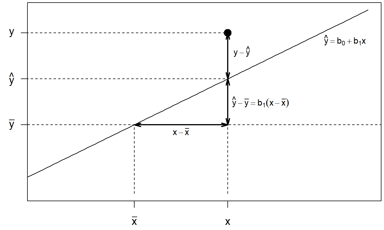
Figure 2.5: Geometric display of the deviation decomposition.
Now, from the algebraic decomposition in equation (2.1), square each side of the equation and sum over all observations. After a little algebraic manipulation, this yields \[\begin{equation} \sum_{i=1}^{n}\left( y_i-\overline{y}\right) ^2=\sum_{i=1}^{n}\left( y_i-\widehat{y}_i\right) ^2+\sum_{i=1}^{n}\left( \widehat{y}_i- \overline{y}\right) ^2. \tag{2.2} \end{equation}\] We rewrite this as \(Total~SS=Error~SS+Regression~SS\) where \(SS\) stands for sum of squares. We interpret:
\(Total~SS\) as the total variation without knowledge of \(x\),
\(Error~SS\) as the total variation remaining after the introduction of \(x\), and
\(Regression~SS\) as the difference between the \(Total~SS\) and \(Error~SS\) , or the total variation “explained” through knowledge of \(x\).
When squaring the right-hand side of equation (2.1), we have the cross-product term \(2\left( y_i-\widehat{y}_i\right) \left( \widehat{y}_i-\overline{y}\right)\). With the “algebraic manipulation,” one can check that the sum of the cross-products over all observations is zero. This result is not true for all fitted lines but is a special property of the least squares fitted line.
In many instances, the variability decomposition is reported through only a single statistic.
Definition. The coefficient of determination is denoted by the symbol \(R^2\), called “\(R\)-square, and defined as \[ R^2=\frac{Regression~SS}{Total~SS}. \]
We interpret \(R^2\) to be the proportion of variability explained by the regression line. In one extreme case where the regression line fits the data perfectly, we have \(Error~SS=0\) and \(R^2=1\). In the other extreme case where the regression line provides no information about the response, we have \(Regression~SS=0\) and \(R^2=0.\) The coefficient of determination is constrained by the inequalities \(0 \leq R^2 \leq 1\) with larger values implying a better fit.
2.3.2 The Size of a Typical Deviation: s
In the basic linear regression model, the deviation of the response from the regression line, \(y_i-\left( \beta_0+\beta_1x_i\right)\), is not an observable quantity because the parameters \(\beta_0\) and \(\beta_1\) are not observed. However, by using estimators \(b_0\) and \(b_1\), we can approximate this deviation using \[ e_i=y_i-\widehat{y}_i=y_i-\left( b_0+b_1x_i\right) , \] known as the residual.
Residuals will be critical to developing strategies for improving model specification in Section 2.6. We now show how to use the residuals to estimate \(\sigma ^2\). From a first course in statistics, we know that if one could observe the deviations \(\varepsilon_i\), then a desirable estimate of \(\sigma ^2\) would be \((n-1)^{-1}\sum_{i=1}^{n}\left( \varepsilon _i-\overline{\varepsilon }\right) ^2\). Because {\(\varepsilon_i\)} are not observed, we use the following.
Definition. An estimator of \(\sigma ^2\), the mean square error (MSE), is defined as \[\begin{equation} s^2=\frac{1}{n-2}\sum_{i=1}^{n}e_i{}^2. \tag{2.3} \end{equation}\] The positive square root, \(s=\sqrt{s^2},\) is called the residual standard deviation.
Comparing the definitions of \(s^2\) and \((n-1)^{-1}\sum_{i=1}^{n}\left( \varepsilon_i-\overline{\varepsilon }\right) ^2\), you will see two important differences. First, in defining \(s^2\) we have not subtracted the average residual from each residual before squaring. This is because the average residual is zero, a special property of least squares estimation (see Exercise 2.14). This result can be shown using algebra and is guaranteed for all data sets.
Second, in defining \(s^2\) we have divided by \(n-2\) instead of \(n-1\). Intuitively, dividing by either \(n\) or \(n-1\) tends to underestimate \(\sigma ^2\). The reason is that, when fitting lines to data, we need at least two observations to determine a line. For example, we must have at least three observations for there to be any variability about a line. How much “freedom” is there for variability about a line? We will say that the error degrees of freedom is the number of observations available, \(n\), minus the number of observations needed to determine a line, 2 (with symbols, \(df=n-2\)). However, as we saw in the least squares estimation subsection, we do not need to identify two actual observations to determine a line. The idea is that if an analyst knows the line and \(n-2\) observations, then the remaining two observations can be determined, without variability. When dividing by \(n-2\), it can be shown that \(s^2\) is an unbiased estimator of \(\sigma ^2\).
We can also express \(s^2\) in terms of the sum of squares quantities. That is,
\[ s^2=\frac{1}{n-2}\sum_{i=1}^{n}\left( y_i-\widehat{y}_i\right) ^2= \frac{Error~SS}{n-2}=MSE. \]
This leads us to the analysis of variance, or ANOVA, table:
\[ \begin{array}{llcl} \hline \hline \text{ANOVA Table} \\ \hline \text{Source} & \text{Sum of Squares} & df & \text{Mean Square} \\ \hline \text{Regression} & Regression~SS & 1 & Regression~MS \\ \text{Error} & Error~SS & n-2 & MSE \\ \text{Total} & Total~SS & n-1 & \\ \hline \hline \end{array} \]
The ANOVA table is merely a bookkeeping device used to keep track of the sources of variability; it routinely appears in statistical software packages as part of the regression output. The mean square column figures are defined to be the sums of square (\(SS\)) figures divided by their respective degrees of freedom (\(df\)). In particular, the mean square for errors (\(MSE\)) equals \(s^2\) and the regression sum of squares equals the regression mean square. This latter property is specific to the regression with one variable case; it is not true where we consider more than one explanatory variable.
The error degrees of freedom in the ANOVA table is \(n-2\). The total degrees of freedom is \(n-1\), reflecting the fact that the total sum of squares is centered about the mean (at least two observations are required for positive variability). The single degree of freedom associated with the regression portion means that the slope, plus one observation, is enough information to determine the line. This is because it takes two observations to determine a line and at least three observations for there to be any variability about the line.
The analysis of variance table for the lottery data is:
| Sum of Squares | \(df\) | Mean Square | |
|---|---|---|---|
| Regression | 2,527,165,015 | 1 | 2,527,165,015 |
| Error | 690,116,755 | 48 | 14,377,432 |
| Total | 3,217,281,770 | 49 |
R Code to Produce Lottery ANOVA Table
From this table, you can check that \(R^2=78.5\%\) and \(s=3,792.\)
Video: Section Summary
2.4 Properties of Regression Coefficient Estimators
The least squares estimates can be expressed as weighted sum of the responses. To see this, define the weights \[ w_i=\frac{x_i-\overline{x}}{s_x^2(n-1)}. \] Because the sum of \(x\)-deviations (\(x_i-\overline{x}\)) is zero, we see that \(\sum_{i=1}^{n}w_i=0\). Thus, we can express the slope estimate \[\begin{equation} b_1=r\frac{s_y}{s_x}=\frac{1}{(n-1)s_x^2}\sum_{i=1}^{n}\left( x_i-\overline{x}\right) \left( y_i-\overline{y}\right) =\sum_{i=1}^{n}w_i\left( y_i-\overline{y}\right) =\sum_{i=1}^{n}w_iy_i. \tag{2.4} \end{equation}\]
The exercises ask the reader to verify that \(b_0\) can also be expressed as a weighted sum of responses, so our discussion pertains to both regression coefficients. Because regression coefficients are weighted sums of responses, they can be affected dramatically by unusual observations (see Section 2.6).
Because \(b_1\) is a weighted sum, it is straightforward to derive the expectation and variance of this statistic. By the linearity of expectations and Assumption F1, we have \[ \mathrm{E}~b_1=\sum_{i=1}^{n}w_i~\mathrm{E}~y_i=\beta_0\sum_{i=1}^{n}w_i+\beta_1\sum_{i=1}^{n}w_ix_i=\beta_1. \] That is, \(b_1\) is an unbiased estimator of \(\beta_1\). Here, the sum \(\sum_{i=1}^{n}w_ix_i\) \(=\) \(\left[ s_x^2(n-1)\right] ^{-1}\sum_{i=1}^{n}\left( x_i-\overline{x}\right) x_i\) \(=\left[s_x^2(n-1)\right] ^{-1}\sum_{i=1}^{n}\left( x_i-\overline{x}\right) ^2=1.\) From the definition of the weights, some easy algebra also shows that \(\sum_{i=1}^{n}w_i^2=1/\left( s_x^2(n-1)\right)\). Further, the independence of the responses implies that the variance of the sum is the sum of the variances, and thus we have \[ \mathrm{Var}~b_1 =\sum_{i=1}^{n}w_i^2\mathrm{Var}~y_i=\frac{\sigma^2}{s_x^2(n-1)}. \] Replacing \(\sigma ^2\) by its estimator \(s^2\) and taking square roots leads to the following.
Definition. The standard error of \(b_1\), the estimated standard deviation of \(b_1\), is defined as \[\begin{equation} se(b_1)=\frac{s}{s_x\sqrt{n-1}}. \tag{2.5} \end{equation}\]
This is our measure of the reliability, or precision, of the slope estimator. Using equation (2.5), we see that \(se(b_1)\) is determined by three quantities, \(n\), \(s\) and \(s_x\), as follows:
- If we have more observations so that \(n\) becomes larger, then $ se(b_1)$ becomes smaller, other things equal.
- If the observations have a greater tendency to lie closer to the line so that \(s\) becomes smaller, then \(se(b_1)\) becomes smaller, other things equal.
- If values of the explanatory variable become more spread out so that $ s_x$ increases, then \(se(b_1)\) becomes smaller, other things equal.
Smaller values of \(se(b_1)\) offer a better opportunity to detect relations between \(y\) and \(x\). Figure 2.6 illustrates these relationships. Here, the scatter plot in the middle has the smallest value of \(se(b_1)\). Compared with the middle plot, the left-hand plot has a larger value of \(s\) and thus \(se(b_1)\). Compared with the right-hand plot, the middle plot has a larger \(s_x\), and thus smaller value of \(se(b_1)\).
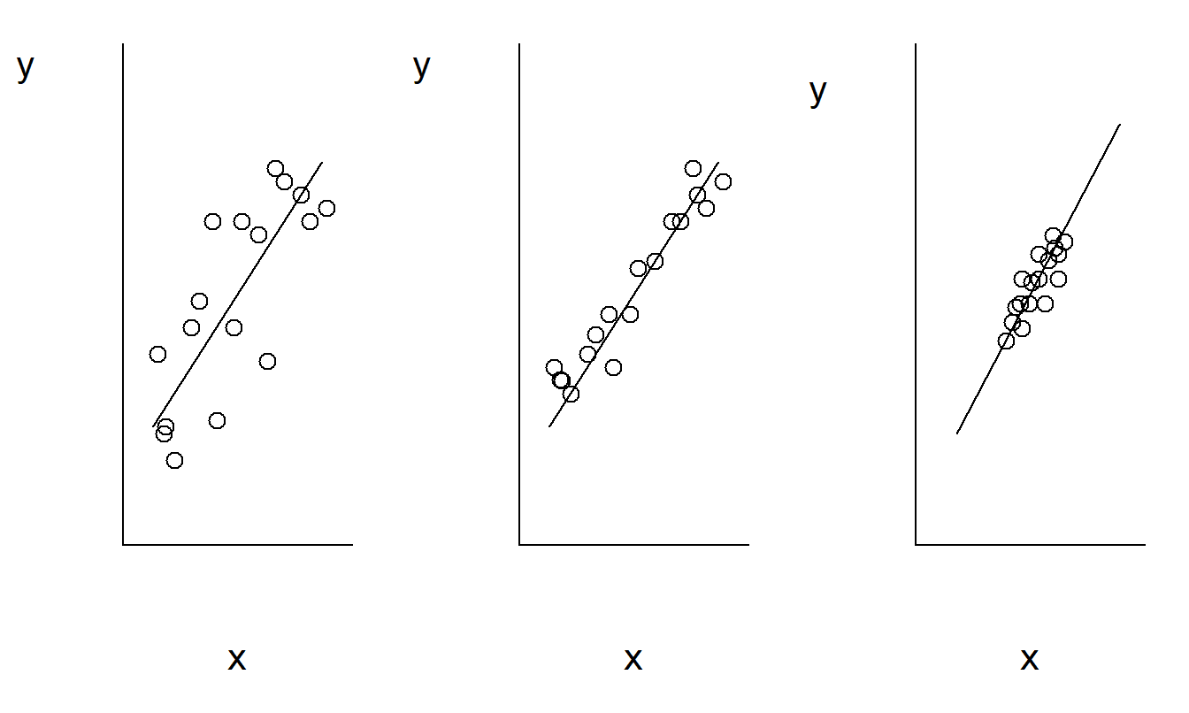
Figure 2.6: These three scatter plots exhibit the same linear relationship between \(y\) and \(x\). The plot on the left exhibits greater variability about the line than the plot in the middle. The plot on the right exhibits a smaller standard deviation in \(x\) than the plot in the middle.
R Code to Produce Figure 2.6
Equation (2.4) also implies that the regression coefficient \(b_1\) is normally distributed. That is, recall from mathematical statistics that linear combinations of normal random variables are also normal. Thus, if Assumption F5 holds, then \(b_1\) is normally distributed. Moreover, several versions of central limit theorems exists for weighted sums (see, for example, Serfling, 1980). Thus, as discussed in Section 1.4, if the responses \(y_i\) are even approximately normally distributed, then it will be reasonable to use a normal approximation for the sampling distribution of \(b_1\). Using \(se(b_1)\) as the estimated standard deviation of \(b_1\), for large values of \(n\) we have that \(\left( b_1-\beta_1\right) /se(b_1)\) has an approximate standard normal distribution. Although we will not prove it here, under Assumption F5 \(\left( b_1-\beta_1\right) /se(b_1)\) follows a $t $-distribution with degrees of freedom \(df=n-2\).
Video: Section Summary
2.5 Statistical Inference
Having fit a model with a data set, we can make a number of important statements. Generally, it is useful to think about these statements in three categories: (i) tests of hypothesized ideas, (ii) estimates of model parameters and (ii) predictions of new outcomes.
2.5.1 Is the Explanatory Variable Important?: The t-Test
We respond to the question of whether the explanatory variable is important by investigating whether or not \(\beta_1=0\). The logic is that if \(\beta_1=0\), then the basic linear regression model no longer includes an explanatory variable \(x\). Thus, we translate our question of the importance of the explanatory variable into a narrower question that can be answered using the hypothesis testing framework. This narrower question is, is \(H_0:\beta_1=0\) valid? We respond to this question by looking at the test statistic:
\[ t-\mathrm{ratio}=\frac{\mathrm{estimator-hypothesized~value~of~parameter}} {\mathrm{standard~error~of~the~estimator}}. \]
For the case of \(H_0:\beta_1=0\) , we examine \(t\)-ratio \(t(b_1)=b_1/se(b_1)\) because the hypothesized value of \(\beta_1\) is 0. This is the appropriate standardization because, under the null hypothesis and the model assumptions described in Section 2.4, the sampling distribution of \(t(b_1)\) can be shown to be the \(t\)-distribution with \(df=n-2\) degrees of freedom. Thus, to test the null hypothesis \(H_0\) against the alternative \(H_{a}:\beta_1\neq 0\), we reject \(H_0\) if favor of \(H_{a}\) if \(|t(b_1)|\) exceeds a \(t\)-value. Here, this \(t\)-value is a percentile from the \(t\)-distribution using \(df=n-2\) degrees of freedom. We denote the significance level as \(\alpha\) and this \(t\)-value as \(t_{n-2,1-\alpha /2}\).
Example: Lottery Sales - Continued. For the lottery sales example, the residual standard deviation is \(s=3,792\). From Table 2.1, we have \(s_x = 11,098\). Thus, the standard error of the slope is \(se(b_1) = 3792/(11098\sqrt{50-1})=0.0488\). From Section 2.1, the slope estimate is \(b_1=0.647\). Thus, the \(t\)-statistic is \(t(b_1) = 0.647/0.0488 = 13.4\). We interpret this by saying that the slope is 13.4 standard errors above zero. For the significance level, we use the customary value of \(\alpha\) = 5%. The 97.5th percentile from a \(t\)-distribution with \(df=50-2=48\) degrees of freedom is \(t_{48,0.975}=2.011\). Because \(|13.4|>2.011\), we reject the null hypothesis that the slope \(\beta_1 = 0\) in favor of the alternative that \(\beta_1 \neq 0\).
Making decisions by comparing a \(t\)-ratio to a \(t\)-value is called a \(t\)-test. Testing \(H_0:\beta_1=0\) versus \(H_{a}:\beta_1\neq 0\) is just one of many hypothesis tests that can be performed, although it is the most common. Table 2.3 outlines alternative decision-making procedures. These procedures are for testing \(H_0:\beta_1 = d\) where \(d\) is a user-prescribed value that may be equal to zero or any other known value. For example, in our Section 2.7 example, we will use \(d=1\) to test financial theories about the stock market.
Table 2.3 Decision-Making Procedures for Testing \(H_0:\beta_1 = d\)
\[ \begin{array}{c|c} \hline \text{Alternative Hypothesis} (H_{a}) & \text{Procedure: Reject } H_0 \text{ in favor of } H_{a} \text{ if} \\ \hline \beta_1>d & t-\mathrm{ratio}>t_{n-2,1-\alpha }. \\ \beta_1<d & t-\mathrm{ratio}<-t_{n-2,1-\alpha }. \\ \beta_1\neq d & |t-\mathrm{ratio}\mathit{|}>t_{n-2,1-\alpha /2}. \\ \end{array} \\ {\small \begin{array}{l} \hline \text{Notes: The significance level is } \alpha . \text{Here, }t_{n-2,1-\alpha} \text{ the } (1-\alpha )th \text{ percentile}\\ ~~\text{from the } t-\text{distribution using } df=n-2 \text{ degrees of freedom}.\\ ~~\text{The test statistic is }t-\mathrm{ratio} = (b_1 -d)/se(b_1) . \\ \hline \end{array} } \]
Alternatively, one can construct probability (\(p\)-) values and compare these to given significant levels. The \(p\)-value is a useful summary statistic for the data analyst to report since it allows the report reader to understand the strength of the deviation from the null hypothesis. Table 2.4 summarizes the procedure for calculating \(p\)-values.
Table 2.4 Probability Values for Testing \(H_0:\beta_1 = d\)
\[ \begin{array}{c|ccc} \hline \text{Alternative} & & & \\ \text{Hypothesis} (H_a) & \beta_1>d & \beta_1<d & \beta_1\neq d \\ \hline p-value & \Pr(t_{n-2}>t-\mathrm{ratio}) & \Pr(t_{n-2}<t-\mathrm{ratio}) & \Pr (|t_{n-2}|>|t-\mathrm{ratio}\mathit{|}) \\\hline \end{array} \\ {\small \begin{array}{l} \hline \text{Notes: Here, }t_{n-2} \text{ is a } t-\text{distributed random variable with } df=n-2 \text{ degrees of freedom.}\\ ~~\text{The test statistic is }t-\mathrm{ratio} = (b_1 -d)/se(b_1) . \\ \hline \end{array} } \]
Another interesting way of addressing the question of the importance of an explanatory variable is through the correlation coefficient. Remember that the correlation coefficient is a measure of linear relationship between \(x\) and \(y\). Let’s denote this statistic by \(r(y,x)\). This quantity is unaffected by scale changes in either variable. For example, if we multiply the \(x\) variable by the number \(b_1\), then the correlation coefficient remains unchanged. Further, correlations are unchanged by additive shifts. Thus, if we add a number, say \(b_0\), to each \(x\) variable, then the correlation coefficient remains unchanged. Using a scale change and an additive shift on the \(x\) variable can be used to produce the fitted value \(\widehat{y}=b_0+b_1x\). Thus, using notation, we have \(|r(y,x)|=r(y,\widehat{y}).\) We may thus interpret the correlation between the responses and the explanatory variable to be equal to the correlation between the responses and the fitted values. This leads then to the following interesting algebraic fact, \(R^2=r^2.\) That is, the coefficient of determination equals the correlation coefficient squared. This is much easier to interpret if one thinks of \(r\) as the correlation between observed and fitted values. See Exercise 2.13 for steps useful in confirming this result.
2.5.2 Confidence Intervals
Investigators often cite the formal hypothesis testing mechanism to respond to the question “Does the explanatory variable have a real influence on the response?” A natural follow-up question is “To what extent does \(x\) affect \(y\)?” To a certain degree, one could respond using the size of the \(t\)-ratio or the \(p\)-value. However, in many instances a confidence interval for the slope is more useful.
To introduce confidence intervals for the slope, recall that \(b_1\) is our point estimator of the true, unknown slope \(\beta_1\). Section 2.4 argued that this estimator has standard error \(se(b_1)\) and that \(\left( b_1-\beta_1\right) /se(b_1)\) follows a \(t\)-distribution with \(n-2\) degrees of freedom. Probability statements can be inverted to yield confidence intervals. Using this logic, we have the following confidence interval for the slope \(\beta_1\).
Definition. A \(100(1-\alpha)\)% confidence interval for the slope \(\beta_1\) is \[\begin{equation} b_1\pm t_{n-2,1-\alpha /2} ~se(b_1). \tag{2.6} \end{equation}\]
As with hypothesis testing, \(t_{n-2,1-\alpha /2}\) is the (1-\(\alpha\)/2)th percentile from the \(t\)-distribution with \(df=n-2\) degrees of freedom. Because of the two-sided nature of confidence intervals, the percentile is 1 - (1 - confidence level) / 2. In this text, for notational simplicity we generally use a 95% confidence interval, so the percentile is 1-(1-0.95)/2 = 0.975. The confidence interval provides a range of reliability that measures the usefulness of the estimate.
In Section 2.1, we established that the least squares slope estimate for the lottery sales example is \(b_1=0.647\). The interpretation is that if a zip code’s population differs by 1,000, then we expect mean lottery sales to differ by $647. How reliable is this estimate? It turns out that \(se(b_1)=0.0488\) and thus an approximate 95% confidence interval for the slope is \[ 0.647\pm (2.011)(.0488), \] or (0.549, 0.745). Similarly, if population differs by 1,000, a 95% confidence interval for the expected change in sales is (549, 745). Here, we use the \(t\)-value \(t_{48,0.975}=2.011\) because there are 48 (= \(n\)-2) degrees of freedom and, for a 95% confidence interval, we need the 97.5th percentile.
2.5.3 Prediction Intervals
In Section 2.1, we showed how to use least squares estimators to predict the lottery sales for a zip code, outside of our sample, having a population of 10,000. Because prediction is such an important task for actuaries, we formalize the procedure so that it can be used on a regular basis.
To predict an additional observation, we assume that the level of explanatory variable is known and is denoted by \(x_{\ast}\). For example, in our previous lottery sales example we used \(x_{\ast} = 10,000\). We also assume that the additional observation follows the same linear regression model as the observations in the sample.
Using our least square estimators, our point prediction is \(\widehat{y}_{\ast} = b_0 + b_1 x_{\ast}\), the height of the fitted regression line at \(x_{\ast}\) We may decompose the prediction error into two parts:
\[ \begin{array}{ccccc} \underbrace{y_{\ast} - \widehat{y}_{\ast}} & = & \underbrace{\beta_0 - b_0 + \left( \beta_1 - b_1 \right) x_{\ast}} & + & \underbrace{\varepsilon_{\ast}} \\ {\small \text{prediction error} }& {\small =} & {\small \text{error in estimating the } }& {\small +} & {\small \text{deviation of the additional } }\\ & & {\small \text{regression line at }x}_{\ast} & & {\small \text{response from its mean}} \end{array} \]
It can be shown that the standard error of the prediction is \[ se(pred) = s \sqrt{1+\frac{1}{n}+\frac{\left( x_{\ast}-\overline{x}\right) ^2}{(n-1)s_x^2}}. \] As with \(se(b_1)\), the terms \(n^{-1}\) and \(\left( x_{\ast}-\overline{x} \right) ^2/\left[ (n-1)s_x^2\right]\) become close to zero as the sample size \(n\) becomes large. Thus, for large \(n\), we have that \(se(pred)\approx s\), reflecting that the error in estimating the regression line at a point becomes negligible and deviation of the additional response from its mean becomes the entire source of uncertainty.
Definition. A \(100(1-\alpha)\)% prediction interval at \(x_{\ast}\) is \[\begin{equation} \widehat{y}_{\ast} \pm t_{n-2,1-\alpha /2} ~se(pred) \tag{2.7} \end{equation}\] where the \(t\)-value \(t_{n-2,1-\alpha /2}\) is the same as used for hypothesis testing and the confidence interval.
For example, the point prediction at \(x_{\ast} = 10,000\) is \(\widehat{y}_{\ast}\)= 469.7 + 0.647 (10000) = 6,939.7. The standard error of this prediction is \[ se(pred) = 3,792 \sqrt{1+\frac{1}{50} + \frac{\left( 10,000-9,311\right)^2}{(50-1)(11,098)^2}} = 3,829.6. \] With a \(t\)-value equal to 2.011, this yields an approximate 95% prediction interval \[ 6,939.7 \pm (2.011)(3,829.6) = 6,939.7 \pm 7,701.3 = (-761.6, ~14,641.0). \] We interpret these results by first pointing out that our best estimate of lottery sales for a zip code with a population of 10,000 is 6,939.70. Our 95% prediction interval represents a range of reliability for this prediction. If we could see many zip codes, each with a population of 10,000, on average we expect about 19 out of 20, or 95%, would have lottery sales between 0 and 14,641. It is customary to truncate the lower bound of the prediction interval to zero if negative values of the response are deemed to be inappropriate.
R Code to Produce Section 2.5 Analyses
Video: Section Summary
2.6 Building a Better Model: Residual Analysis
Quantitative disciplines calibrate models with data. Statistics takes this one step further, using discrepancies between the assumptions and the data to improve model specification. We will examine the Section 2.2 modeling assumptions in light of the data and use any mismatch to specify a better model; this process is known as diagnostic checking (like when you go to a doctor and he or she performs diagnostic routines to check your health).
We will begin with the Section 2.2 error representation. Under this set of assumptions, the deviations {\(\varepsilon_i\)} are identically and independently distributed (i.i.d), and under assumption F5, normally distributed. To assess the validity of these assumptions, one uses (observed) residuals {\(e_i\)} as approximations for the (unobserved) deviations {\(\varepsilon_i\)}. The basic theme is that if the residuals are related to a variable or display any other recognizable pattern, then we should be able to take advantage of this information and improve our model specification. The residuals should contain little or no information and represent only natural variation from the sampling that cannot be attributed to any specific source. Residual analysis is the exercise of checking the residuals for patterns.
There are five types of model discrepancies that analysts commonly look for. If detected, the discrepancies can be corrected with the appropriate adjustments in the model specification.
Model Misspecification Issues
Lack of Independence. There may exist relationships among the deviations {\(\varepsilon_i\)} so that they are not independent.
Heteroscedasticity. Assumption E3 that indicates that all observations have a common (although unknown) variability, known as homoscedasticity. Heteroscedascity is the term used when the variability varies by observation.
Relationships between Model Deviations and Explanatory Variables. If an explanatory variable has the ability to help explain the deviation \(\varepsilon\), then one should be able to use this information to better predict \(y\).
Nonnormal Distributions. If the distribution of the deviation represents a serious departure from normality, then the usual inference procedures are no longer valid.
Unusual Points. Individual observations may have a large effect on the regression model fit, meaning that the results may be sensitive to the impact of a single observation. \end{enumerate}
This list will serve the reader throughout your study of regression analysis. Of course, with only an introduction to basic models we have not yet seen alternative models that might be used when we encounter these model discrepancies. In this book’s Part II on time series models, we will study lack of independence among data ordered over time. Chapter 5 will consider heteroscedasticity in further detail. The introduction to multiple linear regression in Chapter 3 will be our first look at handling relationships between {\(\varepsilon_i\)} and additional explanatory variables. We have, however, already had an introduction to the effect of normal distributions, seeing that \(qq\) plots can detect non-normality and that transformations can help induce approximate normality. In this section, we discuss the effects of unusual points.
Much of residual analysis is done by examining a standardized residual, a residual divided by its standard error. An approximate standard error of the residual is \(s\); in Chapter 3 we will give a precise mathematical definition. There are two reasons why we often examine standardized residuals in lieu of basic residuals. First, if responses are normally distributed, then standardized residuals are approximately realizations from a standard normal distribution. This provides a reference distribution to compare values of standardized residuals. For example, if a standardized residual exceeds two in absolute value, this is considered unusually large and the observation is called an outlier. Second, because standardized residuals are dimensionless, we get carryover of experience from one data set to another. This is true regardless of whether or not the normal reference distribution is applicable.
Outliers and High Leverage Points
Another important part of residual analysis is the identification of unusual observations in a data set. Because regression estimates are weighted averages with weights that vary by observation, some observations are more important than others. This weighting is more important than many users of regression analysis realize. In fact, the example below demonstrates that a single observation can have a dramatic effect in a large data set.
There are two directions in which a data point can be unusual, the horizontal and vertical directions. By “unusual,” we mean that an observation under consideration seems to be far from the majority of the data set. An observation that is unusual in the vertical direction is called an outlier. An observation that is unusual in the horizontal directional is called a high leverage point. An observation may be both an outlier and a high leverage point.
Example: Outliers and High Leverage Points. Consider the fictitious data set of 19 points plus three points, labeled A, B, and C, given in Figure 2.7 and Table 2.5. Think of the first 19 points as “good” observations that represent some type of phenomena. We want to investigate the effect of adding a single aberrant point.
Table 2.5. 19 Base Points Plus Three Types of Unusual Observations
\[ \small{ \begin{array}{c|cccccccccc|ccc} \hline Variables & &&&&&&&&& & A & B & C \\ \hline x & 1.5 & 1.7 & 2.0 & 2.2 & 2.5 & 2.5 & 2.7 & 2.9 & 3.0 & 3.5 & 3.4 & 9.5 & 9.5 \\ y & 3.0 & 2.5 & 3.5 & 3.0 & 3.1 & 3.6 & 3.2 & 3.9 & 4.0 & 4.0 & 8.0 & 8.0 & 2.5 \\ \hline x & 3.8 & 4.2 & 4.3 & 4.6 & 4.0 & 5.1 & 5.1 & 5.2 & 5.5 & & & & \\ y & 4.2 & 4.1 & 4.8 & 4.2 & 5.1 & 5.1 & 5.1 & 4.8 & 5.3 & & & & \\ \hline \end{array} } \]
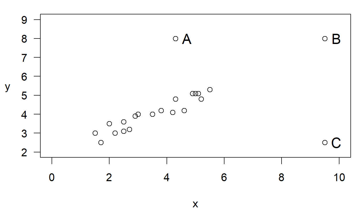
Figure 2.7: Scatterplot of 19 base plus three unusual points, labeled A, B and C.
R Code to Produce Figure 2.7
To investigate the effect of each type of aberrant point, Table 2.6 summarizes the results of four separate regressions. The first regression is for the nineteen base points. The other three regressions use the nineteen base points plus each type of unusual observation.
Table 2.6. Results from Four Regressions
\[ \begin{array}{l|rrrrr} \hline Data & b_0 & b_1 & s & R^2(\%) & t(b_1) \\ \hline 19 \text{ Base Points} & 1.869 & 0.611 & 0.288 & 89.0 & 11.71 \\ 19 \text{ Base Points} ~+~ A & 1.750 & 0.693 & 0.846 & 53.7 & 4.57 \\ 19 \text{ Base Points} ~+~ B & 1.775 & 0.640 & 0.285 & 94.7 & 18.01 \\ 19 \text{ Base Points} ~+~ C & 3.356 & 0.155 & 0.865 & 10.3 & 1.44 \\ \hline \end{array} \]
Table 2.6 shows that a regression line provides a good fit for the nineteen base points. The coefficient of determination, \(R^2\), indicates about 89% of the variability has been explained by the line. The size of the typical error, \(s\), is about 0.29, small compared to the scatter in the \(y\)-values. Further, the \(t\)-ratio for the slope coefficient is large.
When the outlier point A is added to the nineteen base points, the situation deteriorates dramatically. The \(R^2\) drops from 89% to 53.7% and \(s\) increases from about 0.29 to about 0.85. The fitted regression line itself does not change that much even though our confidence in the estimates has decreased.
An outlier is unusual in the \(y\)-value, but “unusual in the \(y\)-value” depends on the \(x\)-value. To see this, keep the \(y\)-value of Point A the same, but increase the \(x\)-value and call the point B.
When the point B is added to the nineteen base points, the regression line provides a better fit. Point B is close to being on the line of the regression fit generated by the nineteen base points. Thus, the fitted regression line and the size of the typical error, \(s\), do not change much. However, \(R^2\) increases from 89% to nearly 95 percent. If we think of \(R^2\) as \(1-(Error~SS)/(Total~SS)\), by adding point B we have increased $ Total~SS$, the total squared deviations in the \(y\)’s, even though leaving \(Error~SS\) relatively unchanged. Point B is not an outlier, but it is a high leverage point.
To show how influential this point is, drop the \(y\)-value considerably and call this the new point C. When this point is added to the nineteen base points, the situation deteriorates dramatically. The \(R^2\) coefficient drops from 89% to 10%, and the \(s\) more than triples, from 0.29 to 0.87. Further, the regression line coefficients change dramatically.
Most users of regression at first do not believe that one point in twenty can have such a dramatic effect on the regression fit. The fit of a regression line can always be improved by removing an outlier. If the point is a high leverage point and not an outlier, it is not clear whether the fit will be improved when the point is removed.
Simply because you can dramatically improve a regression fit by omitting an observation does not mean you should always do so! The goal of data analysis is to understand the information in the data. Throughout the text, we will encounter many data sets where the unusual points provide some of the most interesting information about the data. The goal of this subsection is to recognize the effects of unusual points; Chapter 5 will provide options for handling unusual points in your analysis.
All quantitative disciplines, such as accounting, economics, linear programming, and so on, practice the art of sensitivity analysis. Sensitivity analysis is a description of the global changes in a system due to a small local change in an element of the system. Examining the effects of individual observations on the regression fit is a type of sensitivity analysis.
Example: Lottery Sales – Continued. Figure 2.8 exhibits an outlier; the point in the upper left-hand side of the plot represents a zip code that includes Kenosha, Wisconsin. Sales for this zip code are unusually high given its population. Kenosha is close to the Illinois border; residents from Illinois probably participate in the Wisconsin lottery thus effectively increasing the potential pool of sales in Kenosha. Table 2.7 summarizes the regression fit both with and without this zip code.
Table 2.7. Regression Results with and without Kenosha
\[ \small{ \begin{array}{l|rrrrr} \hline \text{Data} & b_0 & b_1 & s & R^2(\%) & t(b_1) \\ \hline \text{With Kenosha} & 469.7 & 0.647 & 3,792 & 78.5 & 13.26 \\ \text{Without Kenosha} & -43.5 & 0.662 & 2,728 & 88.3 & 18.82 \\ \hline \end{array} } \]
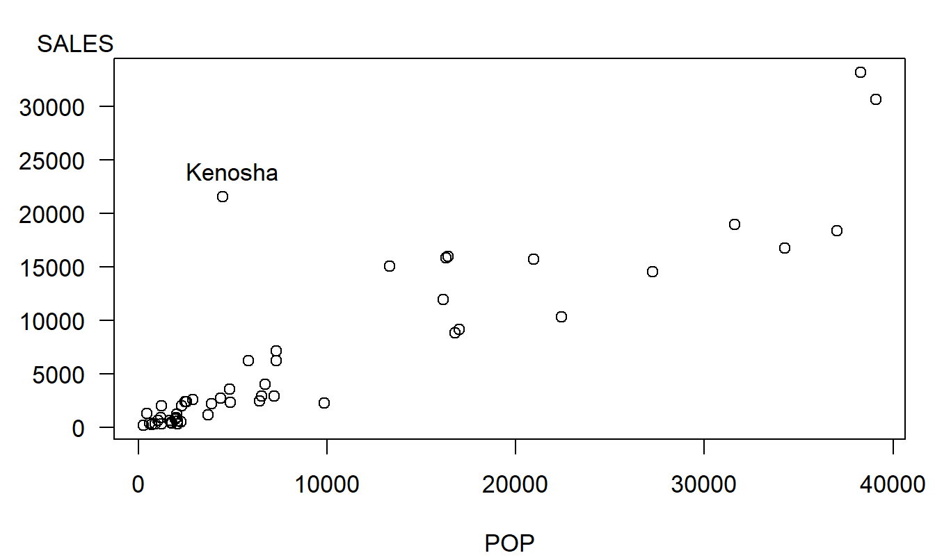
Figure 2.8: Scatter plot of SALES versus POP, with the outlier corresponding to Kenosha marked.
R Code to Produce Figure 2.8 and Table 2.7
For the purposes of inference about the slope, the presence of Kenosha does not alter the results dramatically. Both slope estimates are qualitatively similar and the corresponding \(t\)-statistics are very high, well above cut-offs for statistical significance. However, there are dramatic differences when assessing the quality of the fit. The coefficient of determination, \(R^2\), increased from 78.5% to 88.3% when deleting Kenosha. Moreover, our “typical deviation” \(s\) dropped by over $1,000. This is particularly important if we wish to tighten our prediction intervals.
To check the accuracy of our assumptions, it is also customary to check the normality assumption. One way of doing this is the \(qq\) plot, introduced in Section 1.2. The two panels in Figures 2.9 are \(qq\) plots with and without the Kenosha zip code. Recall that points “close” to linear indicate approximate normality. In the right-hand panel of Figure 2.9, the sequence does appear to be linear so that residuals are approximately normally distributed. This is not the case in the left-hand panel, where the sequence of points appears to climb dramatically for large quantiles. The interesting thing is that the non-normality of the distribution is due to a single outlier, not a pattern of skewness that is common to all the observations.
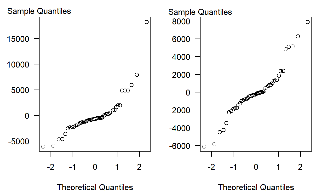
Figure 2.9: \(qq\) Plots of Wisconsin Lottery Residuals. The left-hand panel is based on all 50 points. The right-hand panel is based on 49 points, residuals from a regression after removing Kenosha.
R Code to Produce Figure 2.9
Video: Section Summary
2.7 Application: Capital Asset Pricing Model
In this section, we study a financial application, the Capital Asset Pricing Model, often referred to by the acronym CAPM. The name is something of a misnomer in that the model is really about returns based on capital assets, not the prices themselves. The types of assets that we examine are equity securities that are traded on an active market, such as the New York Stock Exchange (NYSE). For a stock on the exchange, we can relate returns to prices through the following expression:
\[ \small{ \mathrm{return=}\frac{\mathrm{ price~at~the~end~of~a~period+dividends-price~at~the~beginning~of~a~period}}{ \mathrm{price~at~the~beginning~of~a~period}}. } \]
If we can estimate the returns that a stock generates, then knowledge of the price at the beginning of a generic financial period allows us to estimate the value at the end of the period (ending price plus dividends). Thus, we follow standard practice and model returns of a security.
An intuitively appealing idea, and one of the basic characteristics of the CAPM, is that there should be a relationship between the performance of a security and the market. One rationale is simply that if economic forces are such that the market improves, then those same forces should act upon an individual stock, suggesting that it also improve. As noted above, we measure performance of a security through the return. To measure performance of the market, several market indices exist that summarize the performance of each exchange. We will use the “equally-weighted” index of the Standard & Poor’s 500. The Standard & Poor’s 500 is the collection of the 500 largest companies traded on the NYSE, where “large” is identified by Standard & Poor’s, a financial services rating organization. The equally-weighted index is defined by assuming a portfolio is created by investing one dollar in each of the 500 companies.
Another rationale for a relationship between security and market returns comes from financial economics theory. This is the CAPM theory, attributed to Sharpe (1964) and Lintner (1965) and based on the portfolio diversification ideas of Harry Markowitz (1959). Other things equal, investors would like to select a return with a high expected value and low standard deviation, the latter being a measure of risk. One of the desirable properties about using standard deviations as a measure of riskiness is that it is straight-forward to calculate the standard deviation of a portfolio. One only needs to know the standard deviation of each security and the correlations among securities. A notable security is a risk-free one, that is, a security that theoretically has a zero standard deviation. Investors often use a 30-day U.S. Treasury bill as an approximation of a risk-free security, arguing that the probability of default of the U.S. government within 30 days is negligible. Positing the existence of a risk-free asset and some other mild conditions, under the CAPM theory there exists an efficient frontier called the securities market line. This frontier specifies the minimum expected return that investors should demand for a specified level of risk. To estimate this line, we can use the equation \[ \mathrm{E}~r = \beta_0 + \beta_1 r_m \] where \(r\) is the security return and \(r_m\) is the market return. We interpret \(\beta_1 r_m\) as a measure of the amount of security return that is attributed to the behavior of the market.
Testing economic theory, or models arising from any discipline, involves collecting data. The CAPM theory is about ex-ante (before the fact) returns even though we can only test with ex-post (after the fact) returns. Before the fact, the returns are unknown and there is an entire distribution of returns. After the fact, there is only a single realization of the security and market return. Because at least two observations are required to determine a line, CAPM models are estimated using security and market data gathered over time. In this way, several observations can be made. For the purposes of our discussions, we follow standard practice in the securities industry and examine monthly prices.
Data
To illustrate, consider monthly returns over the five year period from January, 1986 to December, 1990, inclusive. Specifically, we use the security returns from the Lincoln National Insurance Corporation as the dependent variable (\(y\)) and the market returns from the index of the Standard & Poor’s 500 Index as the explanatory variable (\(x\)). At the time, the Lincoln was a large, multi-line, insurance company, headquartered in the midwest of the U.S., specifically in Fort Wayne, Indiana. Because it was well known for its’ prudent management and stability, it is a good company to begin our analysis of the relationship between the market and an individual stock.
We begin by interpreting some basic summary statistics, in Table 2.8, in terms of financial theory. First, an investor in the Lincoln will be concerned that the five year average return, \(\overline{y}=0.00510\), is below the return of the market, \(\overline{x}=0.00741\). Students of interest theory recognize that monthly returns can be converted to an annual basis using geometric compounding. For example, the annual return of the Lincoln is \((1.0051)^{12}-1=0.062946\), or roughly 6.29 percent. This is compared to an annual return of 9.26% (= (1\(00((1.00741)^{12}-1\))) for the market. A measure of risk, or volatility, that is used in finance is the standard deviation. Thus, interpret \(s_y\) = 0.0859 \(>\) 0.05254 = \(s_x\) to mean that an investment in the Lincoln is riskier than that of the market. Another interesting aspect of Table 2.8 is that the smallest market return, -0.22052, is 4.338 standard deviations below its average ((-0.22052-0.00741)/0.05254 = -4.338). This is highly unusual with respect to a normal distribution.
| Mean | Median | Standard Deviation | Minimum | Maximum | |
|---|---|---|---|---|---|
| LINCOLN | 0.0051 | 0.0075 | 0.0859 | -0.2803 | 0.3147 |
| MARKET | 0.0074 | 0.0142 | 0.0525 | -0.2205 | 0.1275 |
| Source: Center for Research on Security Prices, University of Chicago |
We next examine the data over time, as is given graphically in Figure 2.10. These are scatter plots of the returns versus time, called time series plots. In Figure 2.10, one can clearly see the smallest market return and a quick glance at the horizontal axis reveals that this unusual point is in October, 1987, the time of the well-known market crash.
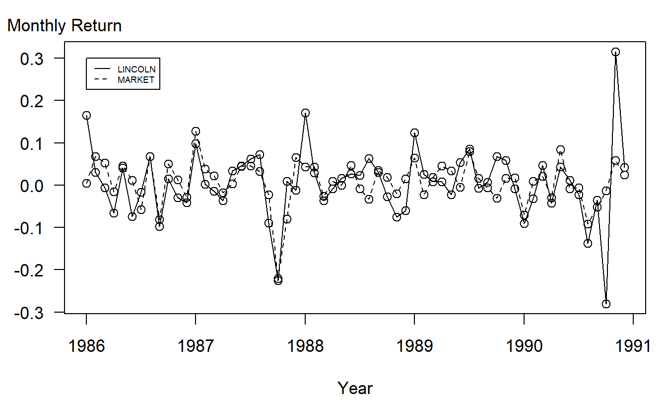
Figure 2.10: Time series plot of returns from the Lincoln National Corporation and the market. There are 60 monthly returns over the period January, 1986 through December, 1990.
The scatter plot in Figure 2.11 graphically summarizes the relationship between Lincoln’s return and the return of the market. The market crash is clearly evident in Figure 2.11 and represents a high leverage point. With the regression line (described below) superimposed, the two outlying points that can be seen in Figure 2.10 are also evident. Despite these anomalies, the plot in Figure 2.11 does suggest that there is a linear relationship between Lincoln and market returns.
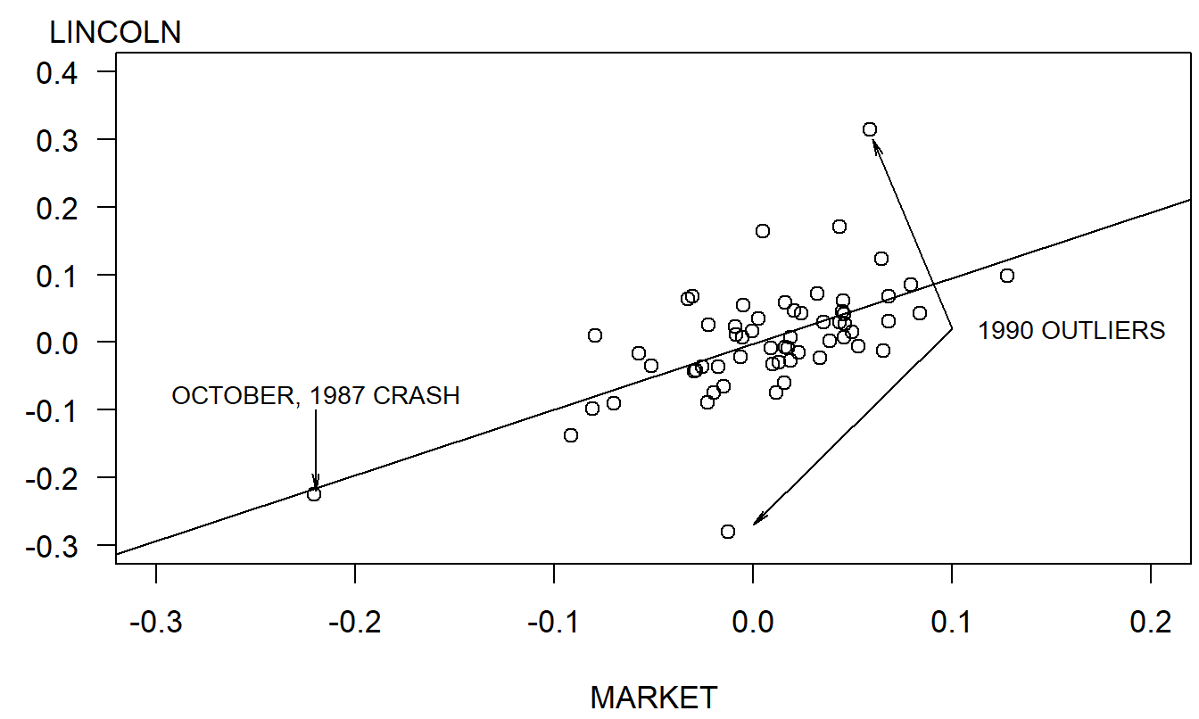
Figure 2.11: Scatterplot of Lincoln’s return versus the S&P 500 Index return. The regression line is superimposed, enabling us to identify the market crash and two outliers.
R Code to Produce Table 2.8 and Figures 2.10 and 2.11
Unusual Points
To summarize the relationship between the market and Lincoln’s return, a regression model was fit. The fitted regression is \[ \widehat{LINCOLN}=-0.00214+0.973 MARKET. \] The resulting estimated standard error, \(s\) = 0.0696 is lower than the standard deviation of Lincoln’s returns, \(s_y=0.0859\). Thus, the regression model explains some of the variability of Lincoln’s returns. Further, the \(t\)-statistic associated with the slope \(b_1\) turns out to be \(t(b_1)=5.64\), which is significantly large. One disappointing aspect is that the statistic \(R^2=35.4\%\) can be interpreted as saying that the market explains only a little over a third of the variability. Thus, even though the market is clearly an important determinant, as evidenced by the high \(t\)-statistic, it provides only a partial explanation of the performance of the Lincoln’s returns.
In the context of the market model, we may interpret the standard deviation of the market, \(s_x\), as non-diversifiable risk. Thus, the risk of a security can be decomposed into two components, the diversifiable component and the market component, which is non-diversifiable. The idea here is that by combining several securities we can create a portfolio of securities that, in most instances, will reduce the riskiness of our holdings when compared with a single security. Again, the rationale for holding a security is that we are compensated through higher expected returns by holding a security with higher riskiness. To quantify the relative riskiness, it is not hard to show that \[\begin{equation} s_y^2 = b_1^2 s_x^2 + s^2 \frac{n-2}{n-1}. \tag{2.8} \end{equation}\]
The riskiness of a security is due to the riskiness due to the market plus the riskiness due to a diversifiable component. Note that the riskiness due to the market component, \(s_x^2\), is larger for securities with larger slopes. For this reason, investors think of securities with slopes \(b_1\) greater than one as “aggressive” and slopes less than one as “defensive.”
Sensitivity Analysis
The above summary immediately raises two additional issues. First, what is the effect of the October, 1987 crash on the fitted regression equation? We know that unusual observations, such as the crash, may potentially influence the fit a great deal. To this end, the regression was re-run without the observation corresponding to the crash. The motivation for this is that the October 1987 crash represents a combination of highly unusual events (the interaction of several automated trading programs operated by the large stock brokerage houses) that we do not wish to represent using the same model as our other observations. Deleting this observation, the fitted regression is \[ \widehat{LINCOLN} = -0.00181 + 0.956 MARKET, \] with \(R^2=26.4\%\), \(t(b_1)=4.52\), \(s=0.0702\) and \(s_y=0.0811\). We interpret these statistics in the same fashion as the fitted model including the October 1987 crash. It is interesting to note, however, that the proportion of variability explained has actually decreased when excluding the influential point. This serves to illustrate an important point. High leverage points are often looked upon with dread by data analysts because they are, by definition, unlike other observations in the data set and require special attention. However, when fitting relationships among variables, they also represent an opportunity because they allow the data analyst to observe the relationship between variables over broader ranges than otherwise possible. The downside is that these relationships may be nonlinear or follow an entirely different pattern when compared to the relationships observed in the main portion of the data.
The second question raised by the regression analysis is what can be said about the unusual circumstances that gave rise to the unusual behavior of Lincoln’s returns in October and November of 1990. A useful feature of regression analysis is to identify and raise the question; it does not resolve it. Because the analysis clearly pinpoints two highly unusual points, it suggests to the data analyst to go back and ask some specific questions about the sources of the data. In this case, the answer is straightforward. In October of 1990, the Travelers’ Insurance Company, a competitor, announced that it would take a large write-off in their real estate portfolio. due to an unprecedented number of mortgage defaults. The market reacted quickly to this news, and investors assumed that other large stock life insurers would also soon announce large write-offs. Anticipating this news, investors tried to sell their portfolios of, for example, Lincoln’s stock, thus causing the price to plummet. However, it turned out that investors overreacted to this news and that Lincoln’s portfolio of real estate was indeed sound. Thus, prices quickly returned to their historical levels.
2.8 Illustrative Regression Computer Output
Computers and statistical software packages that perform specialized calculations play a vital role in modern-day statistical analyses. Inexpensive computing capabilities have allowed data analysts to focus on relationships of interest. Specifying models that are attractive merely for their computational simplicity is much less important now compared to times before the widespread availability of inexpensive computing. An important theme of this text is to focus on relationships of interest and to rely on widely available statistical software to estimate the models that we specify.
With any computer package, generally the most difficult parts of operating the package are the (i) input, (ii) using the commands and (iii) interpreting the output. You will find that most modern statistical software packages accept spreadsheet or text-based files, making input of data relatively easy. Personal computer statistical software packages have menu-driven command languages with easily accessible on-line help facilities. Once you decide what to do, finding the right commands is relatively easy.
This section provides guidance in interpreting the output of
statistical packages. Most statistical packages generate similar
output. Below, three examples of standard statistical software
packages, EXCEL, SAS and R are given. The annotation symbol
“[.]” marks a statistical quantity that is described in the
legend. Thus, this section provides a link between the notation used
in the text and output from some of the standard statistical
software packages.
EXCEL Output
Regression Statistics
Multiple R              0.886283[F]
R Square                0.785497[k]
Adjusted R Square       0.781028[l]
Standard Error          3791.758[j]
Observations              50[a]

ANOVA
           df              SS          MS             F     Significance F
Regression   1[m]   2527165015 [p]  2527165015 [s]  175.773[u]   1.15757E-17[v]
Residual    48[n]   690116754.8[q]  14377432.39[t]
Total       49[o]   3217281770 [r]

        Coefficients    Standard Error      t Stat         P-value
Intercept    469.7036[b] 702.9061896[d]   0.668230846[f] 0.507187[h]
X Variable 1 0.647095[c] 0.048808085[e]   13.25794257[g] 1.16E-17[i]
The SAS System
                         The REG Procedure
                    Dependent Variable: SALES

                        Analysis of Variance
                               Sum of           Mean
Source                   DF        Squares         Square     F Value      Pr > F
Model                  1[m]   2527165015[p]   2527165015[s]   175.77[u]    <.0001[v]
Error                 48[n]    690116755[q]     14377432[t]
Corrected Total       49[o]   3217281770[r]

        Root MSE           3791.75848[j]    R-Square     0.7855[k]
        Dependent Mean     6494.82900[H]    Adj R-Sq     0.7810[l]
        Coeff Var            58.38119[I]

                        Parameter Estimates
                           Parameter       Standard
Variable     Label        DF     Estimate        Error      t  Value    Pr > |t|
Intercept    Intercept     1   469.70360[b]  702.90619[d]    0.67[f]    0.5072[h]
POP          POP           1     0.64709[c]    0.04881[e]   13.26[g]    <.0001[i]
R Output
Analysis of Variance Table

Response: SALES
          Df     Sum Sq      Mean Sq        F value         Pr(>F)
POP        1[m] 2527165015[p] 2527165015[s] 175.77304[u] <2.22e-16[v]***
Residuals 48[n]  690116755[q]   14377432[t]
---
Call: lm(formula = SALES ~ POP)

Residuals:
   Min     1Q Median     3Q    Max
 -6047  -1461   -670    486  18229

Coefficients:
            Estimate     Std. Error t value     Pr(>|t|)
(Intercept) 469.7036[b] 702.9062[d]  0.67[f]    0.51     [h]
POP           0.6471[c]   0.0488[e] 13.26[g]   <2e-16 ***[i]
---
Signif. codes:  0 ?***? 0.001 ?**? 0.01 ?*? 0.05 ?.? 0.1 ? ? 1

Residual standard error: 3792[j] on 48[n] degrees of freedom
Multiple R-Squared: 0.785[k],      Adjusted R-squared: 0.781[l]
F-statistic:  176[u] on 1[m] and 48[n] DF,  p-value: <2e-16[v]
Legend Annotation Definition, Symbol
[a] Number of observations \(n\).
[b] The estimated intercept \(b_0\).
[c] The estimated slope \(b_1\).
[d] The standard error of the intercept, \(se(b_0)\).
[e] The standard error of the slope, \(se(b_1)\).
[f] The \(t\)-ratio associated with the intercept, \(t(b_0) = b_0/se(b_0)\).
[g] The \(t\)-ratio associated with the slope, \(t(b_1) = b_1/se(b_1)\).
[h] The \(p\)-value associated with the intercept; here, \(p-value=Pr(|t_{n-2}|>|t(b_0)|)\), where \(t(b_0)\) is the realized value (0.67 here) and \(t_{n-2}\) has a \(t\)-distribution with \(df=n-2\).
[i] The \(p\)-value associated with the slope; here, \(p-value=Pr(|t_{n-2}|>|t(b_1)|)\), where \(t(b_1)\) is the realized value (13.26 here) and \(t_{n-2}\) has a \(t\)-distribution with \(df=n-2\).
[j] The residual standard deviation, \(s\).
[k] The coefficient of determination, \(R^2\).
[l] The coefficient of determination adjusted for degrees of freedom, \(R_{a}^2\). (This term will be defined in Chapter 3.)
[m] Degree of freedom for the regression component. This is 1 for one explanatory variable.
[n] Degree of freedom for the error component, \(n-2\), for regression with one explanatory variable.
[o] Total degrees of freedoms, \(n-1\).
[p] The regression sum of squares, \(Regression~SS\).
[q] The error sum of squares, \(Error~SS\).
[r] The total sum of squares, \(Total~SS\).
[s] The regression mean square, \(Regression~MS = Regression~SS/1\), for one explanatory variable.
[t] The error mean square, \(s^2=Error~MS = Error~SS/(n-2)\), for one explanatory variable.
[u] The \(F-ratio=(Regression~MS)/(Error~MS)\). (This term will be defined in Chapter 3.)
[v] The \(p\)-value associated with the \(F-ratio\). (This term will be defined in Chapter 3.)
[w] The observation number, \(i\).
[x] The value of the explanatory variable for the \(i\)th observation, \(x_i\).
[y] The response for the \(i\)th observation, \(y_i\).
[z] The fitted value for the \(i\)th observation, \(\widehat{y}_i\).
[A] The standard error of the fit, \(se(\widehat{y}_i)\).
[B] The residual for the \(i\)th observation, \(e_i\).
[C] The standardized residual for the \(i\)th observation, \(e_i/se(e_i)\). The standard error \(se(e_i)\) will be defined in Section 5.3.1.
[F] The multiple correlation coefficient is the square root of the coefficient of determination, \(R=\sqrt{R^2}\). This will be defined in Chapter 3.
[G] The standardized coefficient is \(b_1s_x/s_y\) For regression with one explanatory variable, this is equivalent to \(r\), the correlation coefficient.
[H] The average response, \(\overline{y}\).
[I] The coefficient of variation of the response is \(s_y/\overline{y}\). SAS prints out \(100s_y/\overline{y}\).
2.9 Further Reading and References
Relatively few applications of regression are basic in the sense that they use only one explanatory variable; the purpose of regression analysis is to reduce complex relationships among many variables. Section 2.7 described an important exception to this general rule, the CAPM finance model; see Panjer et al. (1998) for additional actuarial descriptions of this model. Campbell et al. (1997) gives a financial econometrics perspective.
Chapter References
- Anscombe, Frank (1973). Graphs in statistical analysis. The American Statistician 27, 17-21.
- Campbell, John Y., Andrew W. Lo and A. Craig MacKinlay (1997). The Econometrics of Financial Markets. Princeton University Press, Princeton, New Jersey.
- Frees, Edward W. and Tom W. Miller (2003). Sales forecasting using longitudinal data models. International Journal of Forecasting 20, 97-111.
- Goldberger, Arthur (1991). A Course in Econometrics. Harvard University Press, Cambridge.
- Koch, Gary J. (1985). A basic demonstration of the [-1, 1] range for the correlation coefficient. American Statistician 39, 201-202.
- Linter, J. (1965). The valuation of risky assets and the selection of risky investments in stock portfolios and capital budgets. Review of Economics and Statistics, 13-37.
- Manistre, B. John and Geoffrey H. Hancock (2005). Variance of the CTE estimator. North American Actuarial Journal 9(2), 129-156.
- Markowitz, Harry (1959). Portfolio Selection: Efficient Diversification of Investments. John Wiley, New York.
- Panjer, Harry H., Phelim P. Boyle, Samuel H. Cox, Daniel Dufresne, Hans U. Gerber, Heinz H. Mueller, Hal W. Pedersen, Stanley R. Pliska, Michael Sherris, Elias S. Shiu and Ken S. Tan (1998). Financial Economics: With Applications to Investment, Insurance and Pensions. Society of Actuaries, Schaumburg, Illinois.
- Pearson, Karl (1895). Royal Society Proceedings 58, 241.
- Serfling, Robert J. (1980). Approximation Theorems of Mathematical Statistics. John Wiley and Sons, New York.
- Sharpe, William F. (1964). Capital asset prices: A theory of market equilibrium under risk. Journal of Finance, 425-442.
- Stigler, Steven M. (1986). The History of Statistics: The Measurement of Uncertainty before 1900. Harvard University Press, Cambridge, MA.
2.10 Exercises
Sections 2.1-2.2
2.1 Consider the following data set \[ \begin{array}{l|ccc} \hline i & 1 & 2 & 3 \\ \hline x_i & 2 & -6 & 7 \\ y_i & 3 & 4 & 6\\ \hline \end{array} \]
Fit a regression line using the method of least squares. Determine \(r\), \(b_1\) and \(b_0\).
2.2 A perfect relationship, yet zero correlation. Consider the quadratic relationship \(y=x^2\), with data
\[ \begin{array}{l|ccccc} \hline i & 1 & 2 & 3 & 4 & 5\\ \hline x_i & -2 & -1 & 0 & 1 & 2 \\ y_i & 4 & 1 & 0 & 1 & 4\\ \hline \end{array} \]
- Produce a rough graph for this data set.
- Check that the correlation coefficient is \(r=0\).
2.3 Boundedness of the correlation coefficient. Use the following steps to show that \(r\) is bounded by -1 and 1 (These steps are due to Koch, 1990).
- Let \(a\) and \(c\) be generic constants. Verify \[\begin{eqnarray*} 0 & \leq & \frac{1}{n-1}\sum_{i=1}^{n}\left( a\frac{x_i-\overline{x}}{s_x}-c \frac{y_i-\overline{y}}{s_y}\right) ^2 \\ &=& a^2+c^2-2acr. \end{eqnarray*}\]
- Use the results in part (a) to show \(2ac(r-1)\leq (a-c)^2.\)
- By taking \(a=c\), use the result in part (b) to show \(r\leq 1\).
- By taking \(a=-c\), use the results in part (b) to show \(r\geq -1\).
- Under what conditions is \(r=-1\)? Under what conditions is \(r=1\)?
2.4 Regression coefficients are weighted sums. Show that the intercept term, \(b_0\), can be expressed as a weighted sum of the dependent variables. That is, show that \(b_0=\sum_{i=1}^{n}w_{i,0}y_i.\) Further, express the weights in terms of the slope weights, \(w_i\).
2.5 Another expression for the slope as a weighted sum
- Using algebra, establish an alternative expression \[ b_1=\frac{\sum_{i=1}^{n}weight_i~slope_i}{ \sum_{i=1}^{n}weight_i}. \] Here, \(slope_i\) is the slope between \((x_i,y_i)\) and \((\bar{x},\bar{y})\). Give a precise form for the weight \(weight_i\) as a function of the explanatory variable \(x\).
- Suppose that \(\bar{x} = 4,\bar{y} = 3, x_1 = 2 \mathrm{~and~} y_1= 6\). Determine the slope and weight for the first observation, that is, \(slope_1\) and \(weight_1\).
2.6 Consider two variables, \(y\) and \(x\). Do a regression of \(y\) on \(x\) to get a slope coefficient which we call \(b_{1,x,y}\). Do another regression of \(x\) on \(y\) to get a slope coefficient which we call \(b_{1,y,x}\). Show that the correlation coefficient between \(x\) and \(y\) is the geometric mean of the two slope coefficients up to sign, that is, show that \(|r|=\sqrt{ b_{1,x,y}b_{1,y,x}}.\)
2.7 Regression through the origin. Consider the model \(y_i=\beta_1 x_i + \varepsilon_i\), that is, regression with one explanatory variable without the intercept term. This model is called regression through the origin because the true regression line \(\mathrm{E}y = \beta_1 x\) passes through the origin (the point (0, 0)). For this model, the least squares estimate of \(\beta_1\) is that number \(b_1\) that minimizes the sum of squares \(\mathrm{SS}(b_1^{\ast} )=\sum_{i=1}^{n}\left( y_i - b_1^{\ast}x_i\right) ^2.\)
Verify that \[ b_1 = \frac{\sum_{i=1}^{n} x_i y_i}{\sum_{i=1}^{n}x_i^2}. \]
Consider the model \(y_i=\beta_1 z_i^2 + \varepsilon_i\), a quadratic model passing through the origin. Use the result of part
- to determine the least squares estimate of \(\beta_1\).
2.8 a. Show that \[ s_y^2 = \frac{1}{n-1} \sum_{i=1}^{n} \left( y_i-\overline{y} \right)^2 = \frac{1}{n-1} \left( \sum_{i=1}^{n} y_i^2 - n\overline{y}^2 \right) . \]
- Follow the same steps to show \[ \sum_{i=1}^{n}\left( y_i - \overline{y} \right) \left( x_i-\overline{x}\right) =\sum_{i=1}^{n} x_i y_i - n \overline{x}~\overline{y}. \]
- Show that \[ b_{1}= \frac{\sum_{i=1}^{n} \left( y_i-\overline{y}\right) \left( x_i- \overline{x}\right) } {\sum_{i=1}^{n}\left( x_i - \overline{x} \right) ^2} \]
- Establish the commonly used formula \[ b_{1}= \frac{\sum_{i=1}^{n} x_i y_i - n \overline{x} ~ \overline{y} } {\sum_{i=1}^{n} x_i^2 - n \overline{x}^2 }. \]
2.9 Interpretation of coefficients associated with a binary explanatory variable. Suppose that \(x_i\) only takes on the values 0 and 1. Out of the \(n\) observations, \(n_1\) take on the value \(x=0\). These \(n_1\) observations have an average \(y\) value of \(\overline{y}_1\). the remaining \(n-n_1\) observations have value \(x=1\) and an average \(y\) value of \(\overline{y}_2\). Use Exercise 2.8 to show that \(b_1 = \overline{y}_2 - \overline{y}_1.\)
2.10 Nursing Home Utilization. This exercise considers nursing home data provided by the Wisconsin Department of Health and Family Services (DHFS) and described in Exercise 1.2.
Part 1: Use cost report year 2000 data, and do the following analysis.
Correlations
a(i). Calculate the correlation between TPY and LOGTPY. Comment on your result.
a(ii). Calculate the correlation among TPY, NUMBED and SQRFOOT. Do these variables appear highly correlated?
a(iii). Calculate the correlation between TPY and NUMBED/10. Comment on your result.Scatter plots. Plot TPY versus NUMBED and TPY versus SQRFOOT. Comment on the plots.
Basic linear regression.
c(i). Fit a basic linear regression model using TPY as the outcome variable and NUMBED as the explanatory variable. Summarize the fit by quoting the coefficient of determination, \(R^2\), and the \(t\)-statistic for NUMBED.
c(ii). Repeat c(i), using SQRFOOT instead of NUMBED. In terms of \(R^2\), which model fits better?
c(iii). Repeat c(i), using LOGTPY for the outcome variable and LOG(NUMBED) as the explanatory variable.
c(iv). Repeat c(iii), using LOGTPY for the outcome variable and LOG(SQRFOOT) as the explanatory variable.
Part 2: Fit the model in Part 1.c(i) using 2001 data. Are the patterns stable over time?
Sections 2.3-2.4
2.11 Suppose that, for a sample size of \(n\) = 3, you have \(e_2\) = 24 and \(e_{3}\) = -1. Determine \(e_{1}\).
2.12 Suppose that \(r=0\), \(n=15\) and \(s_y = 10\). Determine \(s\).
2.13 The correlation coefficient and the coefficient of determination. Use the following steps to establish a relationship between the coefficient of determination and the correlation coefficient.
- Show that \(\widehat{y}_i-\overline{y}=b_1(x_i-\overline{x}).\)
- Use part (a) to show that \(Regress~SS=\) \(\sum_{i=1}^{n}\left(\widehat{y}_i - \overline{y} \right)^2\) \(= b_1^2s_x^2(n-1).\)
- Use part (b) to establish \(R^2=r^2.\)
2.14 Show that the average residual is zero, that is, show that \(n^{-1}\sum_{i=1}^{n} e_i=0.\)
2.15 Correlation between residuals and explanatory variables.
Consider a generic sequence of pairs of numbers (\(x_1,y_1\)), …,
(\(x_n,y_n\)) with the correlation coefficient computed as
\(r(y,x)=\left[ (n-1)s_ys_x\right] ^{-1}\sum_{i=1}^{n}\left(
y_i-\overline{y}\right) \left( x_i-\overline{x}\right) .\)
- Suppose that either \(\overline{y}=0,\overline{x}=0\) or both \(\overline{x}\) and \(\overline{y}=0.\) Then, check that \(r(y,x)=0\) implies \(\sum_{i=1}^{n}y_i x_i=0\) and vice-versa.
- Show that the correlation between the residuals and the explanatory variables is zero. Do this by using part (a) of Exercise 2.13 to show that \(\sum_{i=1}^{n} x_i e_i = 0\) and then apply part (a).
- Show that the correlation between the residuals and fitted values is zero. Do this by showing that \(\sum_{i=1}^n \widehat{y}_i e_i = 0\) and then apply part (a).
2.16 Correlation and \(t\)-statistics. Use the following steps to establish a relationship between the correlation coefficient and the \(t\)-statistic for the slope.
a Use algebra to check that \[ R^2=1-\frac{n-2}{n-1}\frac{s^2}{s_y^2}. \]
Use part (a) to establish the following quick computational formula for \(s,\) \[s = s_y \sqrt{(1-r^2)\frac{n-1}{n-2}}.\]
Use part (b) to show that \[ t(b_1) = \sqrt{n-2}\frac{r}{\sqrt{1-r^2}}. \]
Sections 2.6-2.7
2.17 Effects of an unusual point. You are analyzing a data set of size \(n=100\). You have just performed a regression analysis using one predictor variable and notice that the residual for the 10th observation is unusually large.
- Suppose that, in fact, it turns out that \(e_{10}=8s\). What percentage of the error sum of squares, \(Error~SS\), is due to the 10th observation?
- Suppose that \(e_{10}=4s\). What percentage of the error sum of squares, \(Error~SS\), is due to the 10th observation?
- Suppose that you reduce the data set to size \(n=20\). After running the regression, it turns out that we still have \(e_{10}=4s\). What percentage of the error sum of squares, \(Error~SS\), is due to the 10th observation?
2.18 Consider a data set consisting of 20 observations with the following summary statistics: \(\overline{x}=0\), \(\overline{y}=9\), \(s_x=1\) and \(s_y=10\). You run a regression using using one variable and determine that \(s=7\). Determine the standard error of a prediction at \(x_{\ast}=1.\)
2.19 Summary statistics can hide important relationships. The data in Table 2.9 is due to Anscombe (1973). The purpose of this exercise is to demonstrate how plotting data can reveal important information that is not evident in numerical summary statistics.
Table 2.9. Anscombe’s (1973) Data
\[ \begin{array}{c|rrrrrr} \hline obs & & & & & & \\ num & x_1 & y_1 & y_2 & y_3 & x_2 & y_4 \\ \hline 1 & 10 & 8.04 & 9.14 & 7.46 & 8 & 6.58 \\ 2 & 8 & 6.95 & 8.14 & 6.77 & 8 & 5.76 \\ 3 & 13 & 7.58 & 8.74 & 12.74 & 8 & 7.71 \\ 4 & 9 & 8.81 & 8.77 & 7.11 & 8 & 8.84 \\ 5 & 11 & 8.33 & 9.26 & 7.81 & 8 & 8.47 \\ 6 & 14 & 9.96 & 8.10 & 8.84 & 8 & 7.04 \\ 7 & 6 & 7.24 & 6.13 & 6.08 & 8 & 5.25 \\ 8 & 4 & 4.26 & 3.10 & 5.39 & 8 & 5.56 \\ 9 & 12 & 10.84 & 9.13 & 8.15 & 8 & 7.91 \\ 10 & 7 & 4.82 & 7.26 & 6.42 & 8 & 6.89 \\ 11 & 5 & 5.68 & 4.74 & 5.73 & 19 & 12.50 \\ \hline \end{array} \]
- Compute the averages and standard deviations of each column of data. Check that the averages and standard deviations of each of the \(x\) columns are the same, within two decimal places, and similarly for each of the \(y\) columns.
- Run four regressions, (1) \(y_{1}\) on \(x_{1}\), (2) \(y_2\) on \(x_{1}\), (3) \(y_{3}\) on \(x_{1}\) and (4) \(y_{4}\) on \(x_2\). Verify, for each of the four regressions fits, that \(b_0\approx 3.0\), \(b_{1}\approx 0.5\), \(s\approx 1.237\) and \(R^2\approx 0.677\), within two decimal places.
- Produce scatter plots for each of the four regression models that you fit in part (b).
- Discuss the fact that the fitted regression models produced in part (b) imply that the four data sets are similar although the four scatter plots produced in part (c) yield a dramatically different story.
2.20 Nursing Home Utilization. This exercise considers nursing home data provided by the Wisconsin Department of Health and Family Services (DHFS) and described in Exercise 1.2 and 2.10.
You decide to examine the relationship between total patient years (LOGTPY) and the number of beds (LOGNUMBED), both in logarithmic units, using cost report year 2001 data.
Summary statistics. Create basic summary statistics for each variable. Summarize the relationship through a correlation statistic and a scatter plot.
Fit the basic linear model. Cite the basic summary statistics, include the coefficient of determination, the regression coefficient for LOGNUMBED and the corresponding \(t\)-statistic.
Hypothesis testing. Test the following hypotheses at the 5% level of significance using a \(t\)-statistic. Also compute the corresponding \(p\)-value.
c(i). Test \(H_0: \beta_1 = 0\) versus \(H_a: \beta_1 \neq 0\).
c(ii). Test \(H_0: \beta_1 = 1\) versus \(H_a: \beta_1 \neq 1\).
c(iii). Test \(H_0: \beta_1 = 1\) versus \(H_a: \beta_1 > 1\).
c(iv). Test \(H_0: \beta_1 = 1\) versus \(H_a: \beta_1 < 1\).You are interested in the effect that a marginal change in LOGNUMBED has on the expected value of LOGTPY.
d(i). Suppose that there is a marginal change in LOGNUMBED of 2. Provide a point estimate of the expected change in LOGTPY.
d(ii). Provide a 95% confidence interval corresponding to the point estimate in part d(i).
d(iii). Provide a 99% confidence interval corresponding to the point estimate in part d(i).At a specified number of beds estimate \(x_{*} = 100\), do these things:
e(i). Find the predicted value of LOGTPY.
e(ii). Obtain the standard error of the prediction.
e(iii). Obtain a 95% prediction interval for your prediction.
e(iv). Convert the point prediction in part e(i) and the prediction interval obtained in part e(iii) into total person years (through exponentiation).
e(v). Obtain a prediction interval as in part e(iv), corresponding to a 90% level (in lieu of 95%).
2.21 Initial Public Offerings. As a financial analyst, you wish to convince a client of the merits of investing in firms that have just entered a stock exchange, as an IPO (initial public offering). Thus, you gather data on 116 firms that priced during the six-month time frame of January 1, 1998 through June 1, 1998. By looking at this recent historical data, you are able to compute RETURN, the firm’s one-year return (in percent).
You are also interested in looking at financial characteristics of the firm that may help you understand (and predict) the return. You initially examine REVENUE, the firm’s 1997 revenues in millions of dollars. Unfortunately, this variable was not available for six firms. Thus, the statistics below are for the 110 firms that have both REVENUES and RETURNS. In addition, Table 2.9 provides information on the (natural) logarithmic revenues, denoted as LnREV, and the initial price of the stock, denoted as PRICEIPO.
| Mean | Median | Standard Deviation | Minimum | Maximum | |
|---|---|---|---|---|---|
| RETURN | 0.106 | -0.130 | 0.824 | -0.938 | 4.333 |
| REV | 134.487 | 39.971 | 261.881 | 0.099 | 1455.761 |
| LnREV | 3.686 | 3.688 | 1.698 | -2.316 | 7.283 |
| PRICEIPO | 13.195 | 13.000 | 4.694 | 4.000 | 29.000 |
You hypothesize that larger firms, as measured by revenues, are more stable and thus should enjoy greater returns. You have determined that the correlation between RETURN and REVENUE is -0.0175.
a(i). Calculate the least squares fit using REVENUE to predict RETURN. Determine \(b_0\) and \(b_1\).
a(ii). For Hyperion Telecommunications, REVENUEs are 95.55 (millions of dollars). Calculate the fitted RETURN using the regression fit in part a(i).
Table 2.11. Regression Results from a Model Fit with Logarithmic Revenues
\[
\begin{array}{l|rrr}
\hline
& & \text{Standard} & \\
\text{Variable} & \text{Coefficient} & \text{Error} & t-\text{statistic} \\
\hline
\text{INTERCEPT} & 0.438 & 0.186 & 2.35\\
\text{LnREV} & -0.090 & 0.046 & -1.97 \\
\hline s = 0.8136, & R^2 = 0.03452 \\ \hline
\end{array}
\]
b. Table 2.11 summarizes a regression using logarithmic revenues and returns.
b(i) Suppose instead that you use LnREVs to predict RETURN.
Calculate the fitted RETURN under this regression model. Is this
equal your answer in part a(ii)?
b(ii) Do logarithmic revenues significantly affect returns? To this end, provide a formal test of hypothesis. State your null and
alternative hypotheses, decision-making criterion and your
decision-making rule. Use a 10% level of significance.
b(iii). You conjecture that, other things equal, that firms with
larger revenues will be more stable and thus enjoy a larger initial
return. Thus, you wish to consider the null hypothesis of no
relation between LnREV and RETURN versus the alternative hypothesis
that there is a positive relation between LnREV and RETURN. To this
end, provide a formal test of hypothesis. State your null and
alternative hypotheses, decision-making criterion and your
decision-making rule. Use a 10% level of significance.
Determine the correlation between LnREV and RETURN. Be sure to state whether this correlation is positive, negative or zero.
You are considering investing in a firm that has LnREV = 2 (so revenues are \(e^2\) = 7.389 millions of dollars).
d(i). Using the fitted regression model, determine the least squares point prediction.
d(ii). Determine the 95% prediction interval corresponding to your prediction in part d(i).The \(R^2\) from the fitted regression model is a disappointing 3.5%. Part of the difficulty is due to observation number 59, the Inktomi Corporation. Inktomi sales are 12th smallest of the data set, with LnREV = 1.76 (so revenues are \(e^{1.76} = 5.79\) millions of dollars), yet it has the highest first year return, with RETURN = 433.33.
e(i). Calculate the residual for this observation.
e(ii). What proportion of the unexplained variability (error sum of squares) does this observation account for?
e(iii). Define the idea of a high leverage observation.
e(iv). Would this observation be considered a high leverage observation? Justify your answer.
2.22 National Life Expectancies. We continue the analysis begun in Exercise 1.7 by examining the relation between \(y= LIFEEXP\) and \(x=FERTILITY\), shown in Figure 2.12. Fit a linear regression model of \(LIFEEXP\) using the explanatory variable \(x=FERTILITY\).
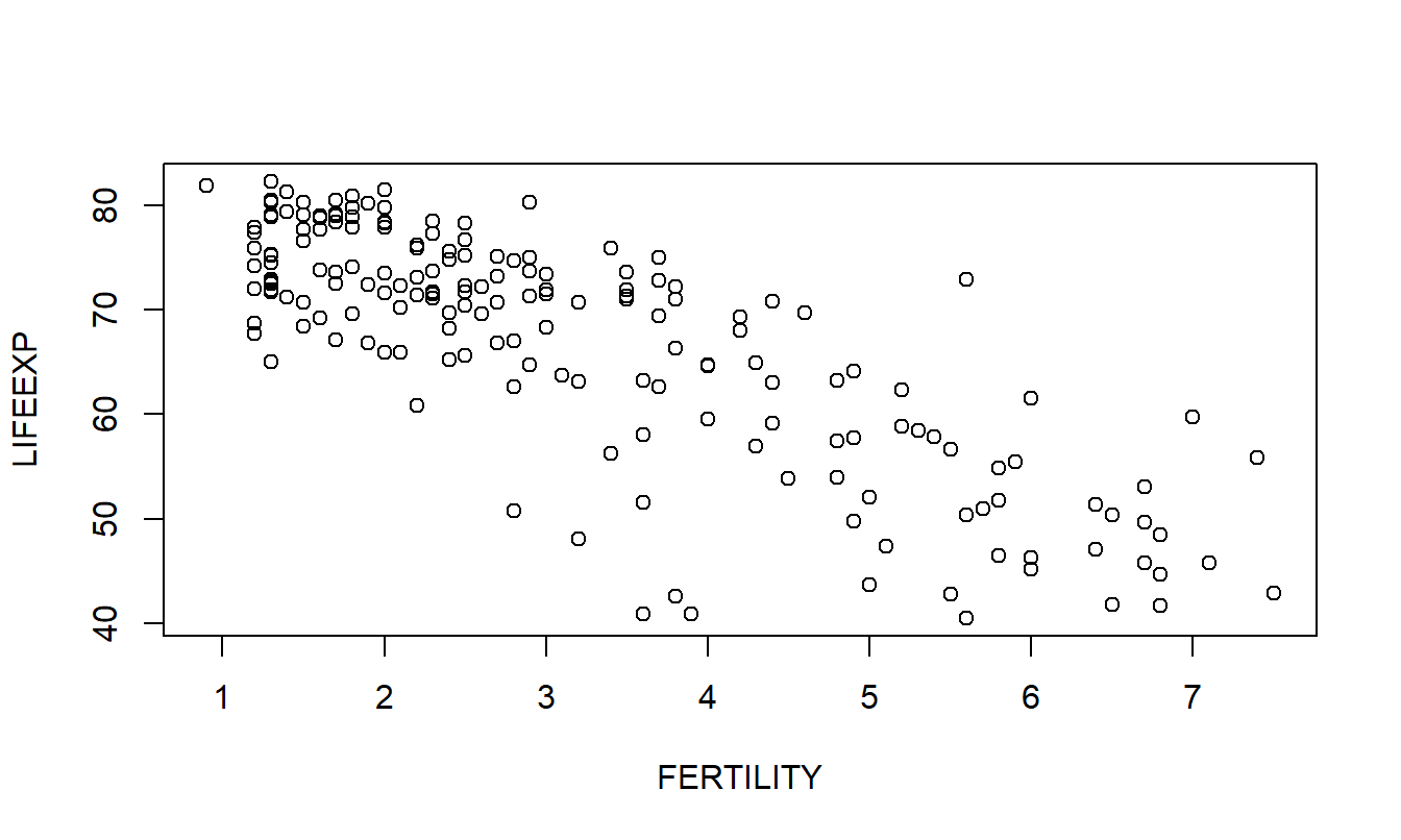
Figure 2.12: Plot of FERTILITY versus LIFEEXP.
- The US has a FERTILITY rate of 2.0. Determine the fitted life expectancy.
- The island nation Dominica did not report a FERTILITY rate and thus was not included in the regression. Suppose that its FERTILITY rate is 2.0. Provide a 95% prediction interval for the life expectancy in Dominica.
- China has a FERTILITY rate of 1.7 and a life expectancy of 72.5. Determine the residual under the model. How many multiples of \(s\) is this residual from zero?
- Suppose that your prior hypothesis is that the FERTILITY slope is -6.0 and you wish to test the null hypothesis that the slope has increased (that is, the slope is greater than -6.0). Test this hypothesis at the 5% level of significance. Also compute an approximate \(p\)-value.
2.11 Technical Supplement - Elements of Matrix Algebra
Examples are an excellent tool for introducing technical topics such as regression. However, this chapter has also used algebra as well as basic probability and statistics to give you further insights into regression analysis. Going forward, we will be studying multivariate relationships. With many things happening concurrently in several dimensions, algebra is no longer useful for providing insights. Instead, we will need matrix algebra. This supplement provides a brief introduction to matrix algebra to allow you to study the linear regression chapters of this text. It re-introduces basic linear regression to give you a feel for things that will be coming up in subsequent chapters when we extend basic linear regression to the multivariate case. Appendix A3 defines additional matrix concepts.
2.11.1 Basic Definitions
A matrix is a rectangular array of numbers arranged in rows and columns (the plural of matrix is matrices). For example, consider the income and age of 3 people. \[ \mathbf{A}= \begin{array}{c} Row~1 \\ Row~2 \\ Row~3 \end{array} \overset{ \begin{array}{cc} ~~~Col~1~ & Col~2 \end{array} }{\left( \begin{array}{cc} 6,000 & 23 \\ 13,000 & 47 \\ 11,000 & 35 \end{array} \right) } \]
Here, column 1 represents income and column 2 represents age. Each row corresponds to an individual. For example, the first individual is 23 years old with an income of $6,000.
The number of rows and columns is called the dimension of the matrix. For example, the dimension of the matrix \(\mathbf{A}\) above is \(3\times 2\) (read 3 “by” 2). This stands for 3 rows and 2 columns. If we were to represent the income and age of 100 people, then the dimension of the matrix would be \(100\times 2\).
It is convenient to represent a matrix using the notation \[ \mathbf{A}=\left( \begin{array}{cc} a_{11} & a_{12} \\ a_{21} & a_{22} \\ a_{31} & a_{32} \end{array} \right) . \] Here, \(a_{ij}\) is the symbol for the number in the \(i\)th row and \(j\)th column of \(\mathbf{A}\). In general, we work with matrices of the form \[ \mathbf{A}=\left( \begin{array}{cccc} a_{11} & a_{12} & \cdots & a_{1k} \\ \vdots & \vdots & \ddots & \vdots \\ a_{n1} & a_{n2} & \cdots & a_{nk} \end{array} \right) . \] In this case, the matrix \(\mathbf{A}\) has dimension \(n\times k\).
A vector is a special matrix. A row vector is a matrix containing only 1 row (\(k=1\)). A column vector is a matrix containing only 1 column (\(n=1\)). For example, \[ \text{column vector}\rightarrow \left( \begin{array}{c} 2 \\ 3 \\ 4 \\ 5 \\ 6 \end{array} \right) ~~~~\text{row vector}\rightarrow \left( \begin{array}{ccccc} 2 & 3 & 4 & 5 & 6 \end{array} \right) . \] Notice above that the row vector takes much less room on a printed page than the corresponding column vector. A basic operation that relates these two quantities is the transpose. The transpose of a matrix \(\mathbf{A}\) is defined by interchanging the rows and columns and is denoted by \(\mathbf{A }^{\prime }\) (or \(\mathbf{A}^{T}\)). For example,
\[ \mathbf{A}=\left( \begin{array}{cc} 6,000 & 23 \\ 13,000 & 47 \\ 11,000 & 35 \end{array} \right) ~~~\mathbf{A}^{\prime }=\left( \begin{array}{ccc} 6,000 & 13,000 & 11,000 \\ 23 & 47 & 35 \end{array} \right) . \] Thus, if \(\mathbf{A}\) has dimension \(n\times k\), then \(\mathbf{A}^{\prime }\) has dimensions \(k\times n\).
2.11.2 Some Special Matrices
A square matrix is a matrix where the number of rows equals the number of columns, that is, \(n=k\).
The diagonal numbers of a square matrix are the numbers of a matrix where the row number equals the column number, for example, \(a_{11}\), \(a_{22}\), and so on. A diagonal matrix is a square matrix where all non-diagonal numbers are equal to 0. For example, \[ \mathbf{A}=\left( \begin{array}{ccc} -1 & 0 & 0 \\ 0 & 2 & 0 \\ 0 & 0 & 3 \end{array} \right) . \]
An identity matrix is a diagonal matrix where all the diagonal numbers are equal to 1. This special matrix is often denoted by \(\mathbf{I}\).
A symmetric matrix is a square matrix \(\mathbf{A}\) such that the matrix remains unchanged if we interchange the roles of the rows and columns. More formally, a matrix \(\mathbf{A}\) is symmetric if \(\mathbf{A=A} ^{\prime }\). For example, \[ \mathbf{A}=\left( \begin{array}{ccc} 1 & 2 & 3 \\ 2 & 4 & 5 \\ 3 & 5 & 10 \end{array} \right) \mathbf{=A}^{\prime }. \] Note that a diagonal matrix is a symmetric matrix.
2.11.3 Basic Operations
Scalar Multiplication
Let \(\mathbf{A}\) by a \(n\times k\) matrix and let \(c\) be a real number. That is, a real number is a \(1\times 1\) matrix and is also called a scalar. Multiplying a scalar \(c\) by a matrix \(\mathbf{A}\) is denoted by \(c\mathbf{A}\) and defined by \[ c\mathbf{A}=\left( \begin{array}{cccc} ca_{11} & ca_{12} & \cdots & ca_{1k} \\ \vdots & \vdots & \ddots & \vdots \\ ca_{n1} & ca_{n2} & \cdots & ca_{nk} \end{array} \right) . \] For example, suppose that \(c=10\) and \[ \mathbf{A}=\left( \begin{array}{cc} 1 & 2 \\ 6 & 8 \end{array} \right) ~~~~ \text{then } ~~~~\mathbf{B}=c\mathbf{A}=\left( \begin{array}{cc} 10 & 20 \\ 60 & 80 \end{array} \right) . \] Note that \(c\mathbf{A}=\mathbf{A}c\).
Addition and Subtraction of Matrices
Let \(\mathbf{A}\) and \(\mathbf{B}\) be matrices with dimensions \(n\times k\). Use \(a_{ij}\) and \(b_{ij}\) to denote the numbers in the \(i\)th row and \(j\)th column of \(\mathbf{A}\) and \(\mathbf{B}\), respectively. Then, the matrix \(\mathbf{C}=\mathbf{A}+\mathbf{B}\) is defined to be the matrix with \((a_{ij}+b_{ij})\) in the \(i\)th row and \(j\)th column. Similarly, the matrix \(\mathbf{C}=\mathbf{A}-\mathbf{B}\) is defined to be the matrix with \((a_{ij}-b_{ij})\) in the \(i\)th row and \(j\)th column. Symbolically, we write this as the following. \[ \text{If }\mathbf{A=}\left( a_{ij}\right) _{ij}\text{ and } \mathbf{B=}\left( b_{ij}\right) _{ij}\text{, then} \] \[ \mathbf{C}=\mathbf{A}+\mathbf{B=}\left( a_{ij}+b_{ij}\right) _{ij}\text{ and }\mathbf{C}=\mathbf{A}-\mathbf{B=}\left( a_{ij}-b_{ij}\right) _{ij}. \] For example, consider \[ \mathbf{A}=\left( \begin{array}{cc} 2 & 5 \\ 4 & 1 \end{array} \right) ~~~\mathbf{B}=\left( \begin{array}{cc} 4 & 6 \\ 8 & 1 \end{array} \right). \] Then \[ \mathbf{A}+\mathbf{B}=\left( \begin{array}{cc} 6 & 11 \\ 12 & 2 \end{array} \right) ~~~\mathbf{A}-\mathbf{B}=\left( \begin{array}{cc} -2 & -1 \\ -4 & 0 \end{array} \right) . \]
Basic Linear Regression Example of Addition and Subtraction. Now, recall that the basic linear regression model can be written as \(n\) equations: \[ \begin{array}{c} y_1=\beta_0+\beta_1x_1+\varepsilon_1 \\ \vdots \\ y_n=\beta_0+\beta_1x_n+\varepsilon_n. \end{array} \] We can define \[ \mathbf{y}=\left( \begin{array}{c} y_1 \\ \vdots \\ y_n \end{array} \right) ~~~\boldsymbol \varepsilon = \left( \begin{array}{c} \varepsilon_1 \\ \vdots \\ \varepsilon_n \end{array} \right) ~~~\text{and}~~~ \mathrm{E~}\mathbf{y} =\left( \begin{array}{c} \beta_0+\beta_1 x_1 \\ \vdots \\ \beta_0 + \beta_1 x_n \end{array} \right) . \] With this notation, we can express the \(n\) equations more compactly as \(\mathbf{y} = \mathrm{E~}\mathbf{y}+\boldsymbol \varepsilon\).
Matrix Multiplication
In general, if \(\mathbf{A}\) is a matrix of dimension \(n\times c\) and $ $ is a matrix of dimension \(c\times k\), then \(\mathbf{C}=\mathbf{AB }\) is a matrix of dimension \(n\times k\) and is defined by \[ \mathbf{C}=\mathbf{AB=}\left( \sum_{s=1}^{c}a_{is}b_{sj}\right) _{ij}. \] For example consider the \(2\times 2\) matrices \[ \mathbf{A}=\left( \begin{array}{cc} 2 & 5 \\ 4 & 1 \end{array} \right) ~~~\mathbf{B}=\left( \begin{array}{cc} 4 & 6 \\ 8 & 1 \end{array} \right) . \] The matrix \(\mathbf{AB}\) has dimension \(2\times 2\). To illustrate the calculation, consider the number in the first row and second column of \(\mathbf{AB}\). By the rule presented above, with \(i=1\) and \(j=2\), the corresponding element of \(\mathbf{AB}\) is \(\sum_{s=1}^2a_{1s}b_{s2}=\) \(a_{11}b_{12}+a_{12}b_{22}=2(6)+5(1)=17\). The other calculations are summarized as \[ \mathbf{AB}=\left( \begin{array}{cc} 2(4)+5(8) & 2(6)+5(1) \\ 4(4)+1(8) & 4(6)+1(1) \end{array} \right) =\left( \begin{array}{cc} 48 & 17 \\ 24 & 25 \end{array} \right) . \] As another example, suppose \[ \mathbf{A}=\left( \begin{array}{ccc} 1 & 2 & 4 \\ 0 & 5 & 8 \end{array} \right) ~~~\mathbf{B}=\left( \begin{array}{c} 3 \\ 5 \\ 2 \end{array} \right) . \] Because \(\mathbf{A}\) has dimension \(2\times 3\) and \(\mathbf{B}\) has dimension \(3\times 1\), this means that the product \(\mathbf{AB}\) has dimension \(2\times 1\).. The calculations are summarized as \[ \mathbf{AB}=\left( \begin{array}{c} 1(3)+2(5)+4(2) \\ 0(3)+5(5)+8(2) \end{array} \right) =\left( \begin{array}{c} 21 \\ 41 \end{array} \right) . \] For some additional examples, we have \[ \left( \begin{array}{cc} 4 & 2 \\ 5 & 8 \end{array} \right) \left( \begin{array}{c} a_1 \\ a_2 \end{array} \right) =\left( \begin{array}{c} 4a_1+2a_2 \\ 5a_1+8a_2 \end{array} \right) . \] \[ \left( \begin{array}{ccc} 2 & 3 & 5 \end{array} \right) \left( \begin{array}{c} 2 \\ 3 \\ 5 \end{array} \right) =2^2+3^2+5^2=38~~~\left( \begin{array}{c} 2 \\ 3 \\ 5 \end{array} \right) \left( \begin{array}{ccc} 2 & 3 & 5 \end{array} \right) =\left( \begin{array}{ccc} 4 & 6 & 10 \\ 6 & 9 & 15 \\ 10 & 15 & 25 \end{array} \right) . \] In general, you see that \(\mathbf{AB\neq BA}\) in matrix multiplication, unlike multiplication of scalars (real numbers). Further, we remark that the identity matrix serves the role of “one” in matrix multiplication, in that \(\mathbf{AI=A}\) and \(\mathbf{IA=A}\) for any matrix \(\mathbf{A}\), providing that the dimensions are compatible to allow matrix multiplication.
Basic Linear Regression Example of Matrix Multiplication. Define \[ \mathbf{X}=\left( \begin{array}{cc} 1 & x_1 \\ \vdots & \vdots \\ 1 & x_n \end{array} \right) \text{ and }\boldsymbol \beta =\left( \begin{array}{c} \beta_0 \\ \beta_1 \end{array} \right) \text{, to get } \mathbf X \boldsymbol \beta =\left( \text{\ } \begin{array}{c} \beta_0+\beta_1x_1 \\ \vdots \\ \beta_0+\beta_1x_n \end{array} \right) =\mathbf{\mathrm{E~}\mathbf{y.}} \] Thus, this yields the familiar matrix expression of the regression model, \(\mathbf{y=X } \boldsymbol \beta + \boldsymbol \varepsilon.\) Other useful quantities include \[ \mathbf{y}^{\prime }\mathbf{y=}\left( \begin{array}{ccc} y_1 & \cdots & y_n \end{array} \right) \left( \begin{array}{c} y_1 \\ \vdots \\ y_n \end{array} \right) =y_1^2+\cdots +y_n^2=\sum_{i=1}^{n}y_i^2, \] \[ \mathbf{X}^{\prime }\mathbf{y=}\left( \begin{array}{ccc} 1 & \cdots & 1 \\ x_1 & \cdots & x_n \end{array} \right) \left( \begin{array}{c} y_1 \\ \vdots \\ y_n \end{array} \right) =\left( \begin{array}{c} \sum_{i=1}^{n}y_i \\ \sum_{i=1}^{n}x_iy_i \end{array} \right) \] and \[ \mathbf{X}^{\prime }\mathbf{X=}\left( \begin{array}{ccc} 1 & \cdots & 1 \\ x_1 & \cdots & x_n \end{array} \right) \left( \begin{array}{cc} 1 & x_1 \\ \vdots & \vdots \\ 1 & x_n \end{array} \right) =\left( \begin{array}{cc} n & \sum_{i=1}^{n}x_i \\ \sum_{i=1}^{n}x_i & \sum_{i=1}^{n} x_i^2 \end{array} \right) . \] Note that \(\mathbf{X}^{\prime }\mathbf{X}\) is a symmetric matrix.
Matrix Inverses
In matrix algebra, there is no concept of “division.” Instead, we extend the concept of “reciprocals” of real numbers. To begin, suppose that \(\mathbf{A}\) is a square matrix of dimension \(k \times k\) and let \(\mathbf{I}\) be the \(k\times k\) identity matrix. If there exists a \(k \times k\) matrix \(\mathbf{B}\) such that \(\mathbf{AB}=\mathbf{I=BA}\), then \(\mathbf{B}\) is called the inverseof \(\mathbf{A}\) and is written \[ \mathbf{B}=\mathbf{A}^{-1}. \] Now, not all square matrices have inverses. Further, even when an inverse exists, it may not be easy to compute by hand. One exception to this rule are diagonal matrices. Suppose that \(\mathbf{A}\) is diagonal matrix of the form \[ \mathbf{A=}\left( \begin{array}{ccc} a_{11} & \cdots & 0 \\ \vdots & \ddots & \vdots \\ 0 & \cdots & a_{kk} \end{array} \right). \text{ Then }\mathbf{A}^{-1}\mathbf{=}\left( \begin{array}{ccc} \frac{1}{a_{11}} & \cdots & 0 \\ \vdots & \ddots & \vdots \\ 0 & \cdots & \frac{1}{a_{kk}} \end{array} \right). \] For example, \[ \begin{array}{cccc} \left( \begin{array}{cc} 2 & 0 \\ 0 & -19 \end{array} \right) & \left( \begin{array}{cc} \frac{1}{2} & 0 \\ 0 & -\frac{1}{19} \end{array} \right) & = & \left( \begin{array}{cc} 1 & 0 \\ 0 & 1 \end{array} \right) \\ \mathbf{A} & \mathbf{A}^{-1} & = & \mathbf{I} \end{array} . \] In the case of a matrix of dimension \(2\times 2\), the inversion procedure can be accomplished by hand easily even when the matrix is not diagonal. In the \(2\times 2\) case, we suppose that if \[ \mathbf{A=}\left( \begin{array}{cc} a & b \\ c & d \end{array} \right), \text{ then }\mathbf{A}^{-1}\mathbf{=}\frac{1}{ad-bc}\left( \begin{array}{cc} d & -b \\ -c & a \end{array} \right) \text{.} \] Thus, for example, if \[ \mathbf{A=}\left( \begin{array}{cc} 2 & 2 \\ 3 & 4 \end{array} \right) \text{ then }\mathbf{A}^{-1}\mathbf{=}\frac{1}{2(4)-2(3)} \left( \begin{array}{cc} 4 & -2 \\ -3 & 2 \end{array} \right) =\left( \begin{array}{cc} 2 & -1 \\ -3/2 & 1 \end{array} \right) \text{.} \] As a check, we have \[ \mathbf{A\mathbf{A}^{-1}=}\left( \begin{array}{cc} 2 & 2 \\ 3 & 4 \end{array} \right) \left( \begin{array}{cc} 2 & -1 \\ -3/2 & 1 \end{array} \right) =\left( \begin{array}{cc} 2(2)-2(3/2) & 2(-1)+2(1) \\ 3(2)-4(3/2) & 3(-1)+4(1) \end{array} \right) =\left( \begin{array}{cc} 1 & 0 \\ 0 & 1 \end{array} \right) =\mathbf{I}\text{.} \]
Basic Linear Regression Example of Matrix Inverses. With \[ \mathbf{X}^{\prime }\mathbf{X=}\left( \begin{array}{cc} n & \sum\limits_{i=1}^{n}x_i \\ \sum\limits_{i=1}^{n}x_i & \sum\limits_{i=1}^{n}x_i^2 \end{array} \right), \] we have \[ \left( \mathbf{X}^{\prime }\mathbf{X}\right) ^{-1}\mathbf{=}\frac{1}{n\sum_{i=1}^{n}x_i^2-\left( \sum_{i=1}^{n}x_i\right) ^2}\left( \begin{array}{cc} \sum\limits_{i=1}^{n}x_i^2 & -\sum\limits_{i=1}^{n}x_i \\ -\sum\limits_{i=1}^{n}x_i & n \end{array} \right). \] To simplify this expression, recall that \(\overline{x}=n^{-1} \sum_{i=1}^{n}x_i\). Thus, \[\begin{equation} \left( \mathbf{X}^{\prime }\mathbf{X}\right) ^{-1}\mathbf{=}\frac{1}{ \sum_{i=1}^{n}x_i^2-n\overline{x}^2}\left( \begin{array}{cc} n^{-1}\sum\limits_{i=1}^{n}x_i^2 & -\overline{x} \\ -\overline{x} & 1 \end{array} \right) . \tag{2.9} \end{equation}\]
Section 3.1 will discuss the relation \(\mathbf{b}=\left( \mathbf{X}^{\prime}\mathbf{X}\right)^{-1} \mathbf{X}^{\prime}\mathbf{y}\). To illustrate the calculation, we have \[\begin{eqnarray*} \mathbf{b} &=&\left( \mathbf{X}^{\prime }\mathbf{X}\right) ^{-1}\mathbf{X} ^{\prime }\mathbf{y=}\frac{1}{\sum_{i=1}^{n}x_i^2-n\overline{x}^2} \left( \begin{array}{cc} n^{-1}\sum\limits_{i=1}^{n}x_i^2 & -\overline{x} \\ -\overline{x} & 1 \end{array} \right) \left( \begin{array}{c} \sum\limits_{i=1}^{n}y_i \\ \sum\limits_{i=1}^{n}x_iy_i \end{array} \right) \\ &=&\frac{1}{\sum_{i=1}^{n}x_i^2-n\overline{x}^2}\left( \begin{array}{c} \sum\limits_{i=1}^{n}\left( \overline{y}x_i^2-\overline{x} x_iy_i\right) \\ \sum\limits_{i=1}^{n}x_iy_i-n\overline{x}\overline{y} \end{array} \right) =\left( \begin{array}{c} b_0 \\ b_1 \end{array} \right) . \end{eqnarray*}\] From this expression, we may see \[ b_1=\frac{\sum\limits_{i=1}^{n}x_iy_i-n\overline{x}\overline{y}}{ \sum\limits_{i=1}^{n}x_i^2-n\overline{x}^2} \] and \[ b_0=\frac{\overline{y}\sum\limits_{i=1}^{n}x_i^2-\overline{x} \sum\limits_{i=1}^{n}x_iy_i}{\sum\limits_{i=1}^{n}x_i^2-n\overline{x} ^2}=\frac{\overline{y}\left( \sum\limits_{i=1}^{n}x_i^2-n\overline{x} ^2\right) -\overline{x}\left( \sum\limits_{i=1}^{n}x_i y_i - n\overline{x} \overline{y}\right) }{\sum\limits_{i=1}^{n}x_i^2-n\overline{x}^2}= \overline{y}-b_1\overline{x}. \] These are the usual expressions for the slope \(b_1\) (Exercise 2.8) and intercept \(b_0\).
2.11.4 Random Matrices
Expectations. Consider a matrix of random variables \[ \mathbf{U=}\left( \begin{array}{cccc} u_{11} & u_{12} & \cdots & u_{1c} \\ u_{21} & u_{22} & \cdots & u_{2c} \\ \vdots & \vdots & \ddots & \vdots \\ u_{n1} & u_{n2} & \cdots & u_{nc} \end{array} \right). \] When we write the expectation of a matrix, this is short-hand for the matrix of expectations. Specifically, suppose that the joint probability function of \({u_{11}, u_{12}, ..., u_{1c}, ..., u_{n1}, ..., u_{nc}}\) is available to define the expectation operator. Then we define \[ \mathrm{E} ~ \mathbf{U} = \left( \begin{array}{cccc} \mathrm{E }u_{11} & \mathrm{E }u_{12} & \cdots & \mathrm{E }u_{1c} \\ \mathrm{E }u_{21} & \mathrm{E }u_{22} & \cdots & \mathrm{E }u_{2c} \\ \vdots & \vdots & \ddots & \vdots \\ \mathrm{E }u_{n1} & \mathrm{E }u_{n2} & \cdots & \mathrm{E }u_{nc} \end{array} \right). \] As an important special case, consider the joint probability function for the random variables \(y_1, \ldots, y_n\) and the corresponding expectations operator. Then \[ \mathrm{E}~ \mathbf{y=} \mathrm{E } \left( \begin{array}{cccc} y_1 \\ \vdots \\ y_n \end{array} \right) = \left( \begin{array}{cccc} \mathrm{E }y_1 \\ \vdots \\ \mathrm{E }y_n \end{array} \right). \] By the linearity of expectations, for a non-random matrix A and vector , we have E ( + ) = E .
Variances. We can also work with second moments of random vectors. The variance of a vector of random variables is called the variance-covariance matrix. It is defined by \[\begin{equation} \mathrm{Var} ~ \mathbf{y} = \mathrm{E} ( (\mathbf{y} - \mathrm{E} \mathbf{y})(\mathbf{y} - \mathrm{E} \mathbf{y})^{\prime} ). \tag{2.10} \end{equation}\] That is, we can express \[ \mathrm{Var}~\mathbf{y=} \mathrm{E } \left( \left( \begin{array}{c} y_1 -\mathrm{E } y_1 \\ \vdots \\ y_n -\mathrm{E } y_n \end{array}\right) \left(\begin{array}{ccc} y_1 - \mathrm{E } y_1 & \cdots & y_n - \mathrm{E } y_n \end{array}\right) \right) \] \[ = \left( \begin{array}{cccc} \mathrm{Var}~y_1 & \mathrm{Cov}(y_1, y_2) & \cdots &\mathrm{Cov}(y_1, y_n) \\ \mathrm{Cov}(y_2, y_1) & \mathrm{Var}~y_2 & \cdots & \mathrm{Cov}(y_2, y_n) \\ \vdots & \vdots & \ddots & \vdots\\ \mathrm{Cov}(y_n, y_1) & \mathrm{Cov}(y_n, y_2) & \cdots & \mathrm{Var}~y_n \\ \end{array}\right), \] because \(\mathrm{E} ( (y_i - \mathrm{E} y_i)(y_j - \mathrm{E} y_j) ) = \mathrm{Cov}(y_i, y_j)\) for \(i \neq j\) and \(\mathrm{Cov}(y_i, y_i) = \mathrm{Var}~y_i\).
In the case that \(y_1, \ldots, y_n\) are mutually uncorrelated, we have that \(\mathrm{Cov}(y_i, y_j)=0\) for \(i \neq j\) and thus \[ \mathrm{Var}~\mathbf{y=} \left( \begin{array}{cccc} \mathrm{Var}~y_1 & 0 & \cdots & 0 \\ 0 & \mathrm{Var}~y_2 & \cdots & 0 \\ \vdots & \vdots & \ddots & \vdots\\ 0 & 0 & \cdots & \mathrm{Var}~y_n \\ \end{array}\right). \] Further, if the variances are identical so that \(\mathrm{Var}~y_i=\sigma ^2\), then we can write \(\mathrm{Var} ~\mathbf{y} = \sigma ^2 \mathbf{I}\), where I is the \(n \times n\) identity matrix. For example, if \(y_1, \ldots, y_n\) are i.i.d., then \(\mathrm{Var} ~\mathbf{y} = \sigma ^2 \mathbf{I}\).
From equation (2.10), it can be shown that \[\begin{equation} \mathrm{Var}\left( \mathbf{Ay +B} \right) = \mathrm{Var}\left( \mathbf{Ay} \right) = \mathbf{A} \left( \mathrm{Var}~\mathbf{y} \right) \mathbf{A}^{\prime}. \tag{2.11} \end{equation}\] For example, if \(\mathbf{A} = (a_1, a_2, \ldots,a_n)= \mathbf{a}^{\prime}\) and B = 0, then equation (2.11) reduces to \[ \mathrm{Var}\left( \sum_{i=1}^n a_i y_i \right) = \mathrm{Var} \left( \mathbf{a^{\prime} y} \right) = \mathbf{a^{\prime}} \left( \mathrm{Var} ~\mathbf{y} \right) \mathbf{a} = (a_1, a_2, \ldots,a_n) \left( \mathrm{Var} ~\mathbf{y} \right) \left(\begin{array}{c} a_1 \\ \vdots \\ a_n \end{array}\right) \] \[ = \sum_{i=1}^n a_i^2 \mathrm{Var} ~y_i ~+~2 \sum_{i=2}^n \sum_{j=1}^{i-1} a_i a_j \mathrm{Cov}(y_i, y_j). \]
Definition - Multivariate Normal Distribution. A vector of random variables \(\mathbf{y} = \left(y_1, \ldots, y_n \right)^{\prime}\) is said to be multivariate normal if all linear combinations of the form \(\sum_{i=1}^n a_i y_i\) are normally distributed. In this case, we write \(\mathbf{y} \sim N (\mathbf{\boldsymbol \mu}, \mathbf{\Sigma} )\), where \(\mathbf{\boldsymbol \mu} = \mathrm{E}~ \mathbf{y}\) is the expected value of y and \(\mathbf{\Sigma}= \mathrm{Var}~\mathbf{y}\) is the variance-covariance matrix of y. From the definition, we have that \(\mathbf{y}\sim N (\mathbf{\boldsymbol \mu}, \mathbf{\Sigma} )\) implies that \(\mathbf{a^{\prime}y}\sim N (\mathbf{a^{\prime} \boldsymbol \mu}, \mathbf{a^{\prime}\Sigma a})\). Thus, if \(y_i\) are i.i.d., then \(\sum_{i=1}^n a_i y_i\) is distributed normally with mean \(\mu \sum_{i=1}^n a_i\) and variance \(\sigma ^2 \sum_{i=1}^n a_i ^2\).