Chapter 14 Survival Models
Chapter Preview. This chapter introduces regression where the dependent variable is the time until an event, such as the time until death, onset of a disease or the default on a loan. Event times are often limited by sampling procedures and so ideas of censoring and truncation of data are summarized in this chapter. Event times are non-negative and their distributions are described in terms of survival and hazard functions. Two types of hazard-based regression are considered, a fully parametric accelerated failure time model and a semi-parametric proportional hazards models.
14.1 Introduction
In survival models, the dependent variable is the time until an event of interest. The classic example of an event is time until death (the complement of death being survival). Survival models are now widely applied in many scientific disciplines; other examples of events of interest include the onset of Alzheimer’s disease (biomedical), time until bankruptcy (economics) and time until divorce (sociology).
Example: Time until Bankruptcy. Shumway (2001) examined the time to bankruptcy for 3,182 firms listed on Compustat Industrial File and the CRSP Daily Stock Return File for the New York Stock Exchange over the period 1962-1992. Several explanatory financial variables were examined, including working capital to total assets, retained earnings to total assets, earnings before interest and taxes to total assets, market equity to total liabilities, sales to total assets, net income to total assets, total liabilities to total assets and current assets to current liabilities. The data set included 300 bankruptcies from 39,745 firm years.
See also Kim et al. (1995) for a similar study on insurance insolvencies.
A distinguishing feature of survival modeling is that it is common for the dependent variable to be observed only in a limited sense. Some events of interest, such as bankruptcy or divorce, never occur for specific subjects (and so can be thought of as taking an infinite time). For other subjects, even when the event time is finite, it may occur after the study period so that the data are (right) censored. That is, complete information about event times may not be available due to the design of the study. Moreover, firms may merge with or be acquired by other firms and individuals may move from a geographical area, leaving the study. Thus, the data may be limited by events that are extraneous to the research question under consideration, represented as random censoring. Censoring is a regular feature of survival data; large values of a dependent variable require more time to develop so that they can be more difficult to observe than small values, other things being equal. Other types of limitations may also occur; subjects whose observation depends on the experience of the event of interest are said to be truncated. To illustrate, in an investigation of old-age mortality, only those who survive to age 85 are recruited to be a part of the study. Section 14.2 describes censoring and truncation in more detail.
Another distinguishing feature of survival modeling is that the dependent variable is positive-valued. Thus, normal curve approximations used in linear regression are less helpful in survival analysis; this chapter introduces alternative regression models. Further, it is customary to interpret models of survival using the hazard function, defined as \[\begin{eqnarray*} \mathrm{h}(t)&= &\frac{probability~density~function} {survival~function} =\frac{\mathrm{f}(t)}{\mathrm{S}(t)}, \end{eqnarray*}\] the “instantaneous” probability of an event, conditional on survivorship up to time \(t\). The hazard function goes by many other names: it is known as the force of mortality in actuarial science, the failure rate in engineering and the intensity function in stochastic processes.
In economics, hazard functions are used to describe duration dependence, the relation between the instantaneous event probability (the density) and the time spent in a given state. Negative duration dependence is associated with decreasing hazard rates. For example, the longer the time until a claimant requests a payment from an insured injury, the lower is the probability of making a request. Positive duration dependence is associated with increasing hazard rates. For example, old-age human mortality generally displays an increasing hazard rate. The older someone is, the higher the near-term probability of death.
A related quantity of interest is the cumulative hazard function, \(H(t)= \int_0^t h(s)ds\). This quantity can also be expressed as the negative log survival function, and conversely, \(\Pr(y>t)=\mathrm{S}(t) = \exp (-H(t))\).
The two most widely used regression models in survival analysis are based on hazard functions. Section 14.3 introduces the accelerated failure time model, where one assumes a linear model for the logarithmic time to failure but with an error distribution that need not be approximately normal. Section 14.4 introduces the the proportional hazards model due to Cox (1972), where one assumes that the hazard function can be written as the product of a “baseline” hazard and a function of a linear combination of explanatory variables.
With survival data we observe a cross-section of subjects where time is the dependent variable of interest. As with Chapter 10 on longitudinal and panel data, there are also applications in which we are interested in repeated observations for each subject. For example, if you are injured in an accident that is covered by insurance, the payments that arise from this claim can occur repeatedly over time, depending on the time to recovery. Section 14.5 introduces the notion of repeated event times, called recurrent events.
14.2 Censoring and Truncation
14.2.1 Definitions and Examples
Two types of limitations encountered in survival data are censoring and truncation. Censoring and truncation are also common features in other actuarial applications, including the Chapter 16 two-part and Chapter 17 fat-tailed models. Thus, this section describes these concepts in detail.
For censoring, the most common form is right-censoring, in which we observe the smaller of the “true” dependent variable and a censoring time variable. For example, suppose that we wish to study the time until a new employee leaves the firm and that we have five years of data to conduct our analysis. Then, we observe the smaller of five years and the amount of time that the employee was with the firm. We also observe whether or not the employee has departed within five years.
Using notation, let \(y\) denote the time to the event, such as the amount of time the employee worked with a firm. Let \(C_U\) denote the censoring time, such as \(C_U=5\). Then, we observe the variable \(y_U^{\ast}= \min(y, C_U)\). We also observe whether or not censoring has occurred. Let \(\delta_U= \mathrm{I}(y \geq C_U)\) be a binary variable that is 1 if censoring occurs, \(y \geq C_U\), and 0 otherwise. For example, in Figure 14.1, values of \(y\) that are greater than the “upper” censoring limit \(C_U\) are not observed – thus, this is often called right-censoring.
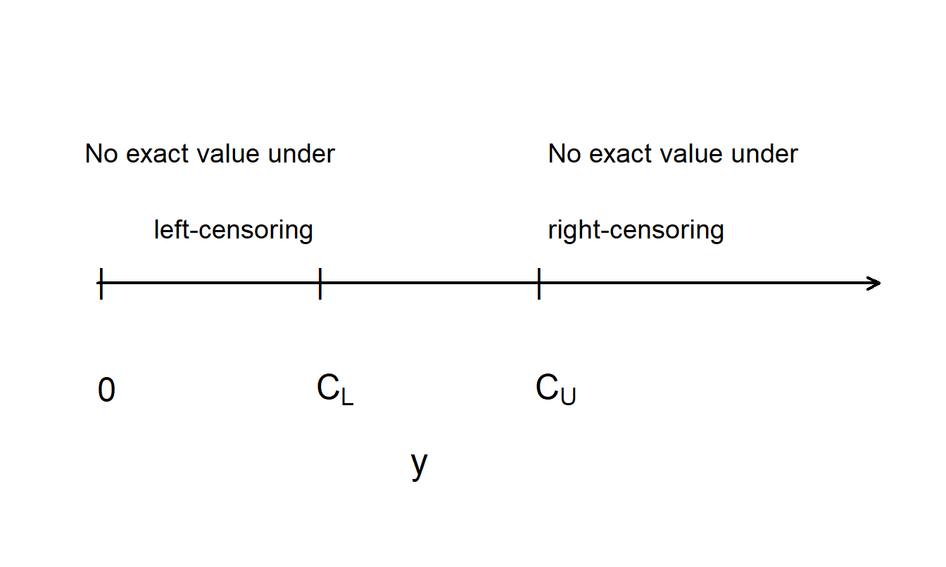
Figure 14.1: Figure Illustrating Left and Right Censoring
Other common forms of censoring are left-censoring and interval censoring. With left-censoring, we observe \(y_L^{\ast}= \max(y, C_L)\) and \(\delta_L= \mathrm{I}(y \leq C_L)\) where \(C_L\) is the censoring time. For example, if you are conducting a study and interviewing a person about an event in the past, the subject may recall that the event occurred before \(C_L\) but not the exact date.
With interval censoring, there is an interval of time, such as \((C_L, C_U)\), in which \(y\) is known to occur but the exact value is not observed. For example, you may be looking at two successive years of annual employee records. People employed in the first year but not the second have left sometime during the year. With an exact departure date, you could compute the amount of time that they were with the firm. Without the departure date, then you only know that they departed sometime during a year-long interval.
Censoring times such as \(C_L\) and \(C_U\) may or may not be stochastic. If the censoring times represent variables known to the analyst, such as the observation period, they are said to be fixed censoring times. Here, the adjective “fixed” means that the times are known in advance. Censoring times may vary by individual but still be fixed. However, censoring may also be the result of an unforeseen phenomena, such as firm merger or a subject moving from a geographical area. In this case, the censoring \(C\) is represented by a random variable and said to be random censoring. If the censoring is fixed or if the random censoring time is independent of the event of interest, then the censoring is said to be non-informative. If the censoring times are independent of the event of interest, then we can essentially treat the censoring as fixed. When censoring and the time to event are dependent (known as informative censoring), then special models are required. For example, if the event of interest is time until bankruptcy of a firm and the censoring mechanism involves filing adequate financial statements, then there is a potential relationship. Financially weak firms are more likely to become bankrupt and less likely to go through the accounting effort to file adequate statements.
Censored observations are available for study, although in a limited form. In contrast, truncated responses are a type of missing data. To illustrate, with left-truncated data, if \(y\) is less than a threshold (say, \(C_L\)), then it is not observed. For right-truncated data, if \(y\) exceeds a threshold (say, \(C_U\)), then it is not observed. To compare truncated and censored observations, consider the following example.
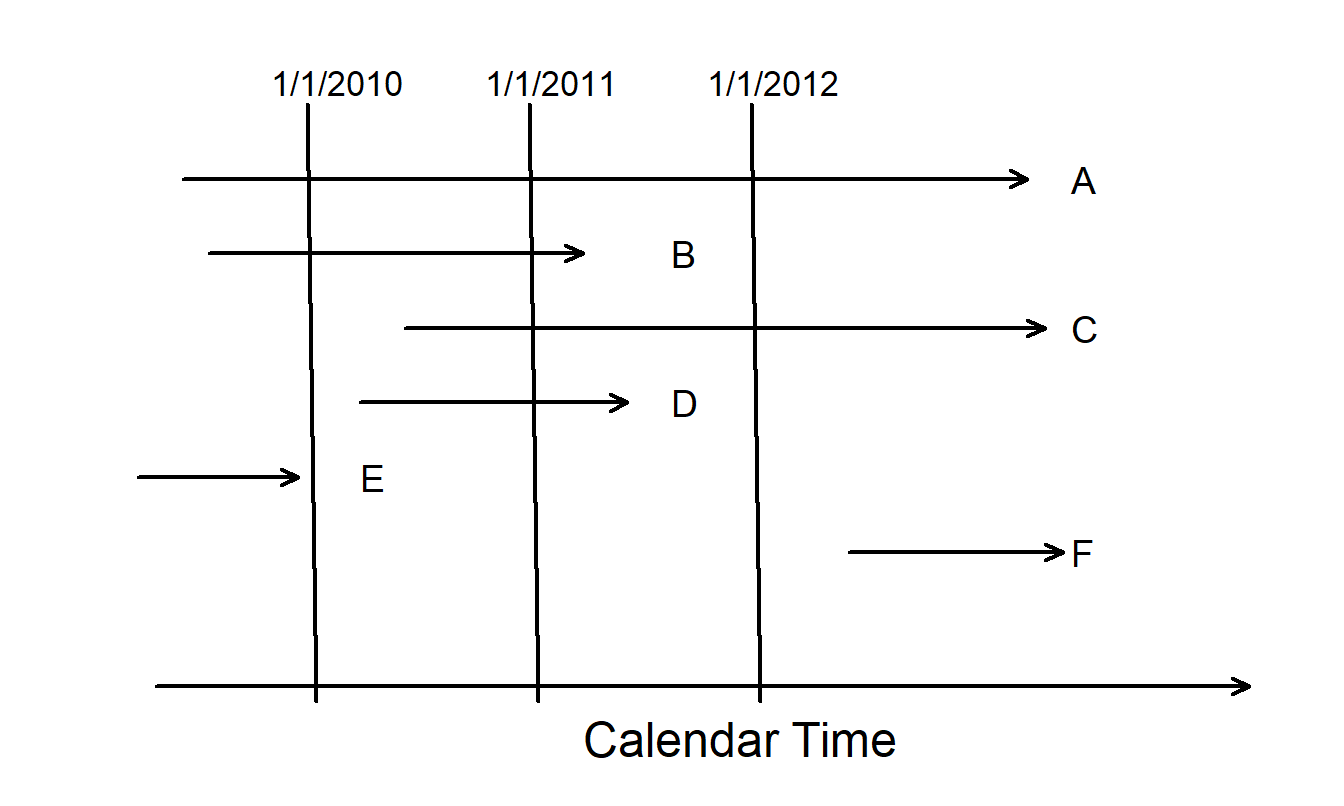
Figure 14.2: Timeline for Several Subjects in a Mortality Study.
Example: Mortality Study. Suppose that you are conducting a two-year study of mortality of high-risk subjects, beginning January 1, 2010 and finishing January 1, 2012. Figure 14.2 graphically portrays the six types of subjects recruited. For each subject, the beginning of the arrow represents that the the subject was recruited and the arrow end represents the event time. Thus, the arrow represents exposure time.
- Type A - right-censored. This subject is alive at the beginning and the end of the study. Because the time of death is not known by the end of the study, it is right-censored. Most subjects are Type A.
- Type B. Complete information is available for a type B subject. The subject is alive at the beginning of the study and the death occurs within the observation period.
- Type C - right-censored and left-truncated. A type C subject is right-censored, in that death occurs after the observation period. However, the subject entered after the start of the study and is said to have a delayed entry time. Because the subject would not have been observed had death occurred before entry, it is left-truncated.
- Type D - left-truncated. A type D subject also has delayed entry. Because death occurs within observation period, this subject is not right censored.
- Type E - left-truncated. A type E subject is not included in the study because death occurs prior to the observation period.
- Type F - right-truncated. Similarly, a type F subject is not included because the entry time occurs after the observation period.
14.2.2 Likelihood Inference
Many inference techniques for survival modeling involve likelihood estimation, so it is helpful to understand the implications of censoring and truncation when specifying likelihood functions. For simplicity, we assume fixed censoring times and a continuous time to event \(y\).
To begin, consider the case of right-censored data where we observe \(y_U^{\ast}= \min(y, C_U)\) and \(\delta_U= \mathrm{I}(y \geq C_U)\). If censoring occurs so that \(\delta_U=1\), then \(y \geq C_U\) and the likelihood is \(\Pr(y \geq C_U) = \mathrm{S}(C_U)\). If censoring does not occur so that \(\delta_U=0\), then \(y < C_U\) and the likelihood is \(\mathrm{f}(y)\). Summarizing, we have \[\begin{eqnarray*} Likelihood &=& \left\{ \begin{array}{cl} \mathrm{f}(y) & \textrm{if}~\delta=0 \\ \mathrm{S}(C_U) & \textrm{if}~\delta=1 \end{array} \right. \\&=& \left( \mathrm{f}(y)\right)^{1-\delta} \left( \mathrm{S}(C_U)\right)^{\delta} . \end{eqnarray*}\] The right-hand expression allows us to present the likelihood more compactly. Now, for an independent sample of size \(n\), \(\{ (y_{U1}, \delta_1), \ldots,(y_{Un}, \delta_n) \}\), the likelihood is \[ \prod_{i=1}^n \left( \mathrm{f}(y_i)\right)^{1-\delta_i} \left( \mathrm{S}(C_{Ui})\right)^{\delta_i} = \prod_{\delta_i=0} \mathrm{f}(y_i) \prod_{\delta_i=1} \mathrm{S}(C_{Ui}), \] with potential censoring times \(\{ C_{U1}, \ldots,C_{Un} \}\). Here, the notation “\(\prod_{\delta_i=0}\)” means take the product over uncensored observations, and similarly for “\(\prod_{\delta_i=1}\).”
Truncated data are handled in likelihood inference via conditional probabilities. Specifically, we adjust the likelihood contribution by dividing by the probability that the variable was observed. Summarizing, we have the following contributions to the likelihood for six types of outcomes.
\[ \small{ \begin{array}{lc} \hline \text{Outcome } & \text{Likelihood Contribution} \\\hline \text{Exact value} & f(y) \\ \text{Right censoring} & S(C_U) \\ \text{Left censoring} & 1-S(C_L) \\ \text{Right truncation} & f(y)/(1-S(C_U)) \\ \text{Left truncation} & f(y)/S(C_L) \\ \text{Interval censoring} & S(C_L)-S(C_U) \\ \hline \end{array} } \]
For known event times and censored data, the likelihood is \[ \prod_{E} \mathrm{f}(y_i) \prod_{R} \mathrm{S}(C_{Ui}) \prod_{L} (1-\mathrm{S}(C_{Li})) \prod_{I} (\mathrm{S}(C_{Li})-\mathrm{S}(C_{Ui})), \] where “\(\prod_{E}\)” is the product over observations with Exact values, and similarly for Right-, Left- and Interval-censoring.
For right-censored and left-truncated data, the likelihood is \[ \prod_{E} \frac{\mathrm{f}(y_i)}{\mathrm{S}(C_{Li})} \prod_{R} \frac{\mathrm{S}(C_{Ui})}{\mathrm{S}(C_{Li})} , \] and similarly for other combinations. To get further insights, consider the following.
Special Case: Exponential Distribution. Consider data that are right-censored and left-truncated, with dependent variables \(y_i\) that are exponentially distributed with mean \(\mu\). With these specifications, recall that \(\mathrm{f}(y) = \mu^{-1} \exp(-y/\mu)\) and \(\mathrm{S}(y) = \exp(-y/\mu)\).
For this special case, the logarithmic likelihood is \[ \begin{array}{ll} \ln Likelihood &= \sum_{E} \left( \ln \mathrm{f}(y_i) - \ln \mathrm{S}(C_{Li}) \right) +\sum_{R}\left( \ln \mathrm{S}(C_{Ui})- \ln \mathrm{S}(C_{Li}) \right) \\ &= \sum_{E} (-\ln \mu -(y_i-C_{Li})/\mu ) -\sum_{R} (C_{Ui}-C_{Li})/\mu . \end{array} \] To simplify the notation, define \(\delta_i = \mathrm{I}(y_i \geq C_{Ui})\) to be a binary variable that indicates right-censoring. Let \(y_i^{\ast \ast} = \min(y_i, C_{Ui}) - C_{Li}\) be the amount that the observed variable exceeds the lower truncation limit. With this, the logarithmic likelihood is \[\begin{equation} \ln Likelihood = - \sum_{i=1}^n ((1-\delta_i) \ln \mu + \frac{y_i^{\ast \ast}}{\mu} ). \tag{14.1} \end{equation}\] Taking derivatives with respect to the parameter \(\mu\) and setting it equal to zero yields the maximum likelihood estimator \[\begin{eqnarray*} \widehat{\mu} &=& \frac{1}{n_u} \sum_{i=1}^n y_i^{\ast \ast}, \end{eqnarray*}\] where \(n_u = \sum_i (1-\delta_i)\) is the number of uncensored observations.
14.2.3 Product-Limit Estimator
It can be useful to calibrate likelihood methods with nonparametric methods that do not rely on a parametric form of the distribution. The product-limit estimator due to Kaplan and Meier (1958) is a well-known estimator of the distribution in the presence of censoring.
To introduce this estimator, we consider the case of right-censored data. Let \(t_1 < \cdots < t_c\) be distinct time points at which an event of interest occurs and let \(d_j\) be the number of events at time point \(t_j\). Further, define \(R_j\) to be the corresponding “risk set” - this is the number of observations that are active at an instant just prior to \(t_j\). Using notation, the risk set is \(R_j = \sum_{i=1}^n I\left( y_i \geq t_j \right)\). With this notation, the product-limit estimator of the survival function is \[\begin{equation} \widehat{S}(t) = \left\{ \begin{array}{ll} 1 & t<t_1 \\ \prod_{t_j \leq t} \left(1 - \frac{d_j}{R_j} \right) & t \geq t_1 \end{array} \right. . \tag{14.2} \end{equation}\]
To interpret the product-limit estimator, we look to evaluating it at event times. At the first event time \(t_1\), the estimator is \(\widehat{S}(t_1)= 1- d_1/R_1=(R_1 - d_1)/R_1\), the proportion of non-events from the risk set \(R_1\). At the second event time \(t_2\), the survival probability conditional on survivorship to time \(t_1\) is \(\widehat{S}(t_2)/ \widehat{S}(t_1)= 1 - d_2/R_2=(R_2 - d_2)/R_2\), the proportion of non-events from the risk set \(R_2\). Similarly, at the \(j\)th event time,
\[ \frac{\widehat{S}(t_j)}{\widehat{S}(t_{j-1})}= 1 - \frac{d_j}{R_j}=\frac{R_j - d_j}{R_j} . \] Starting from these conditional probabilities, one can build the survival estimate as
\[ \widehat{S}(t_j) = \frac{\widehat{S}(t_j)}{\widehat{S}(t_{j-1})} \times \cdots \times \frac{\widehat{S}(t_2)}{\widehat{S}(t_{1})} \times \widehat{S}(t_{1}), \] resulting in equation (14.2). In this sense, the estimator is a “product,” up to the time “limit.” For times between event times, the survival estimate is taken to be a constant.
To see how to use the product-limit estimator, we consider a small data set of \(n=23\) observations, where 18 are event times and 5 have been right-censored. This example is from Miller (1997), where the events correspond to survival for patients with acute myelogenous leukemia. After patients received chemotherapy to achieve complete remission, they were randomly allocated to one of two groups, those who received maintenance chemotherapy and those who did not (the control group). The event was time in weeks to relapse from the complete remission state. For those in the maintenance group, the times are: 9, 13, 13+, 18, 23, 28+, 31, 34, 45+, 48, 161+. For those in the control group, the times are: 5, 5, 8, 8, 12, 16+, 23, 27, 30, 33, 43 45. Here, the plus sign (+) indicates right-censoring of an observation.
Figures 14.3 and 14.4 show the product-limit survival function estimates for these data. Notice the step nature of the function, where drops (from the left, or jumps from the right) correspond to event times. When no censoring is involved, the product-limit estimator reduces to the usual empirical estimator of the survival function.
In the figures, censored observations are depicted with a plus (+) plotting symbol. When the last observation has been censored as in Figure 14.3, there are different methods for defining the survival curve for times exceeding this observation. Analysts making estimates at these times will need to be aware of the option that their statistical package uses. The options are described in standard books on survival analysis, such as Klein and Moschberger (1997).
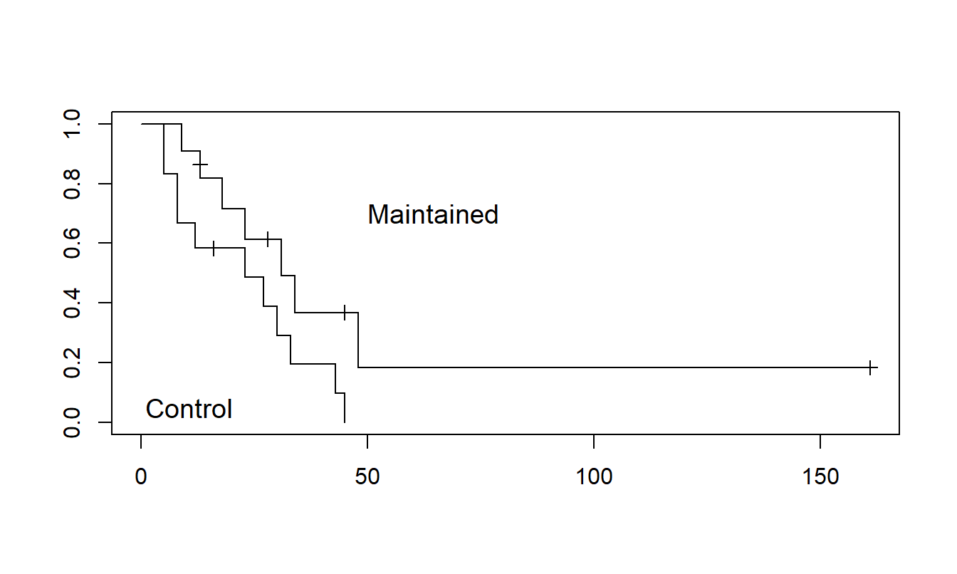
Figure 14.3: Product-Limit Estimate of the Survival Functions for Two Groups. This graph shows that those with maintained chemotherapy treatment have higher estimated survival probabilities than those in the control group.
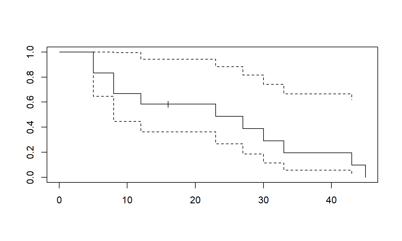
Figure 14.4: Product-Limit Estimate of the Survival Function for the Control Group. The upper and lower bounds are from Greenwood’s formula for the estimate of the variance.
Figure 14.4 also shows an estimate of the standard error. These are calculated using Greenwood’s (1926) formula for an estimate of the variance, given by \[ \widehat{\mathrm{Var}(\widehat{S}(t))} = (\widehat{S}(t))^2 \sum_{t_j \leq t} \frac{d_j}{R_j(R_j-d_j)} . \]
R Code to Produce Figures 14.3 and 14.4
14.3 Accelerated Failure Time Model
An accelerated failure time (\(AFT\)) model can be expressed using a linear regression equation \(\ln y_i = \mathbf{x}_i^{\prime} \boldsymbol \beta + \varepsilon_i\), where \(y_i\) is the event time. Unlike the usual linear regression model, the AFT model makes a parametric assumption about the disturbance term, such as a normal, extreme-value or logistic distribution. As we have seen, the normal distribution is the basis for usual linear regression model. Thus, many analysts begin by taking logarithms of event data and using the usual linear regression routines to explore their data.
Location-Scale Distributions
To understand the name “accelerated failure,” also known as accelerated hazards, it is helpful to review the statistical idea of location-scale families. A parametric location-scale distribution is one where the density function is of the form \[ \mathrm{f}(t) =\frac{1}{\sigma }\mathrm{f}_0 \left( \frac{t-\mu }{\sigma }\right) , \] where \(\mu\) is the location parameter and \(\sigma >0\) is the scale parameter. The case \(\mu =0\) and \(\sigma =1\) corresponds to the standard form of the distribution. Within a location-scale distribution, additive shifts, such as going from degrees Kelvin to degrees Centigrade, \(^{\circ }K=\) \(^{\circ }C+273.15\), and scalar multiples, such as going from dollars to thousands of dollars, remain in the same distribution family. As we will see in Chapter 17, a location parameter is a natural place to introduce regression covariates.
A random variable \(y\) is said to have a log location-scale distribution if \(\ln y\) has a location-scale distribution. Suppose that a random variable \(y_0\) has a standard form location-scale distribution with survival function \(\mathrm{S}_0\left( z\right)\). Then, the survival function of \(y\) defined by \(\ln y = \mu + \sigma y_0\) can be expressed as \[ \mathrm{S}\left( t\right) =\Pr \left( y>t\right) =\Pr \left( y_0>\frac{\ln t-\mu }{\sigma }\right) =\mathrm{S}_0\left( \frac{\ln t-\mu }{\sigma } \right) =\mathrm{S}_0^{\ast }\left( \left( \frac{t}{e^{\mu }}\right) ^{1/\sigma }\right) , \] where \(\mathrm{S}_0^{\ast }(t) =\mathrm{S}_0( \ln t)\) is the survival function of the standard form of \(\ln y\). In the context of survival modeling where \(t\) represents time, the effect of rescaling by dividing by \(e^{\mu }\) can be thought of as “accelerating time” (when \(e^{\mu }<1\)). This is the motivation for the name “accelerated failure time models.” Table 14.1 provides some special cases of widely used location-scale distributions and their log location-scale counterparts.
| Standard Form Survival Distribution | Location-Scale Distribution | Log Location-Scale Distribution |
|---|---|---|
| \(\mathrm{S}_0(t) = \exp(- e^t)\) | Extreme value distribution | Weibull |
| \(\mathrm{S}_0(t) =1 - \Phi(t)\) | Normal | Lognormal |
| \(\mathrm{S}_0(t) = (1 + e^t)^{-1}\) | Logistic | Log-logistic |
Inference for AFT Models
To get an idea of the complexities in estimating an \(AFT\) model, we return to the exponential distribution. This is a special case of Weibull regression with the scale parameter \(\sigma =1\).
Special Case: Exponential Distribution - Continued. To introduce regression covariates, we let \(\mu_i = \exp (\mathbf{x}_i^{\prime} \boldsymbol \beta)\). Using the same reasoning as with equation (14.1), the logarithmic likelihood is \[ \begin{array}{ll} \ln Likelihood &= - \sum_{i=1}^n ((1-\delta_i) \ln \mu_i +\frac{y_i^{\ast \ast}}{\mu_i} )\\ &= - \sum_{i=1}^n ((1-\delta_i) \mathbf{x}_i^{\prime} \boldsymbol \beta+ y_i^{\ast \ast}\exp (-\mathbf{x}_i^{\prime} \boldsymbol \beta)) , \end{array} \] where \(\delta_i = I(y_i \geq C_{Ui})\) and \(y_i^{\ast \ast} =\min(y_i, C_{Ui}) - C_{Li}\). Taking derivatives with respect to \(\boldsymbol \beta\) yields the score function \[ \begin{array}{ll} \frac{\partial \ln Likelihood}{\partial \boldsymbol \beta} &= - \sum_{i=1}^n ((1-\delta_i) \mathbf{x}_i - \mathbf{x}_i y_i^{\ast \ast}\exp (-\mathbf{x}_i^{\prime} \boldsymbol \beta)) \\ &= \sum_{i=1}^n \mathbf{x}_i \frac{y_i^{\ast \ast}-\mu_i (1-\delta_i)} {\mu_i } . \end{array} \] This has the form of a generalized estimating equation, introduced in Chapter 13. Although closed-form solutions rarely exist, it can readily be solved by modern statistical packages.
As this special case illustrates, estimation of \(AFT\) regression models can be readily addressed through maximum likelihood. Moreover, properties of maximum likelihood estimates are well-understood and so we readily have general inference tools, such as estimation and hypothesis testing, available. Standard statistical packages provide output that supports this inference.
14.4 Proportional Hazards Model
The assumption of proportional hazards is defined in Section 14.4.1 and inference techniques are discussed in Section 14.4.2.
14.4.1 Proportional Hazards
In the proportional hazards (\(PH\)) model due to Cox (1972), one assumes that the hazard function can be written as the product of some “baseline” hazard and a function of a linear combination of explanatory variables. To illustrate, we use \[\begin{equation} h_i(t) = h_0(t) \exp( \mathbf{x}_i^{\prime} \boldsymbol \beta ). \tag{14.3} \end{equation}\] where \(h_0(t)\) is the baseline hazard. This is known as a “proportional” hazards model because if one takes the ratio of hazard functions for two sets of covariates, say \(\mathbf{x}_1\) and \(\mathbf{x}_2\), one gets \[ \frac{h_1(t|\mathbf{x}_1)}{h_2(t|\mathbf{x}_1)} = \frac {h_0(t) \exp( \mathbf{x}_1^{\prime} \boldsymbol \beta )} {h_0(t) \exp( \mathbf{x}_2^{\prime} \boldsymbol \beta )} = \exp( (\mathbf{x}_1-\mathbf{x}_2)^{\prime}\boldsymbol \beta ) . \] Note that the ratio does not depend on time \(t\).
As we have seen in many regression applications, users are interested in variable effects and not always concerned with other aspects of the model. The reason that the \(PH\) model in equation (14.3) has proved so popular is that it specifies the explanatory variable effects as a simple function of the linear combination while permitting a flexible baseline component, \(h_0\). Although this baseline is common to all subjects, it need not be specified parametrically as with \(AFT\) models. Further, one need not use the “exp” function for the explanatory variables; however, this is the common specification as it ensures that the hazard function will remain non-negative.
Proportional hazards can be motivated as an extension of exponential regression. Consider a random variable \(y^{\ast}\) that has an exponential distribution with mean \(\mu = \exp (\mathbf{x}^{\prime} \boldsymbol \beta)\). Suppose that we observe \(y = \mathrm{g}(y^{\ast})\), where g(\(\cdot\)) is unknown except that it is monotonically increasing. Many survival distributions are transformations of the exponential distribution. For example, if \(y = \mathrm{g}(y^{\ast})=(y^{\ast})^{\sigma}\), then it is easy to check that \(y\) has a Weibull distribution given in Table 14.1. The Weibull distribution is the only \(AFT\) model that has proportional hazards (see Lawless, 2003, exercise 6.1).
Straight-forward calculations show that the hazard function of \(y\) can be expressed as \[ \mathrm{h}_y(t) = \mathrm{g}^{\prime}(t) / \mu = \mathrm{g}^{\prime}(t) \exp (- \mathbf{x}^{\prime} \boldsymbol \beta ), \] see, for example, Zhou (2001). This has a proportional hazards structure, as in equation (14.3), with \(\mathrm{g}^{\prime}(t)\) serving as the baseline hazard. In the \(PH\) model, the baseline hazard is assumed unknown. In contrast, for the Weibull and other \(AFT\) regression models, the baseline hazard function is assumed known up to one or two parameters that can be estimated from the data.
14.4.2 Inference
Because of the flexible specification of the baseline component, the usual maximum likelihood estimation techniques are not available to estimate the \(PH\) model. To outline the estimation procedure, we let \((y_1, \delta_1), \ldots, (y_n, \delta_n)\) be independent and assume that \(y_i\) follows equation (14.3) with regressors \(\mathbf{x}_i\). That is, we now drop the asterisk (\(\ast\)) notation and let \(y_i\) denote observed values (exact or censored) and use \(\delta_i\) to be the binary variable that indicates (right) censoring. Further, let \(H_0\) be the cumulative hazard function associated with the baseline function \(h_0\). Recalling the general relationship \(\mathrm{S}(t) = \exp (-H(t))\), with equation (14.3) we have \(\mathrm{S}(t) = \exp \left(-H_0(t)\exp( \mathbf{x}_i^{\prime} \boldsymbol \beta )\right).\)
Starting from the usual likelihood perspective, from Section 14.2.2 the likelihood is \[\begin{eqnarray*} L(\boldsymbol \beta , h_0)&= & \prod_{i=1}^n \mathrm{f}(y_i)^{1-\delta_i} \mathrm{S}(y_i)^{\delta_i} = \prod_{i=1}^n h(y_i)^{1-\delta_i} \exp(-H(y_i)) \\ &= & \prod_{i=1}^n \left( h_0(t) \exp( \mathbf{x}_i^{\prime} \boldsymbol \beta ) \right)^{1-\delta_i} \exp\left(-H_0(y_i)\exp( \mathbf{x}_i^{\prime} \boldsymbol \beta ) \right) . \end{eqnarray*}\] Now, parameter estimates that maximize \(L(\boldsymbol \beta , h_0)\) do not follow the usual properties of maximum likelihood estimation because the baseline hazard \(h_0\) is not specified parametrically. One way to think about this problem is due to Breslow (1974) who showed that a nonparametric maximum likelihood estimator of \(h_0\) could be used in \(L(\boldsymbol \beta , h_0)\). This results in what Cox called a partial likelihood, \[\begin{equation} L_P(\boldsymbol \beta) = \prod_{i=1}^n \left( \frac{\exp( \mathbf{x}_i^{\prime} \boldsymbol \beta )} {\sum_{j \in R(y_i)} \exp( \mathbf{x}_j^{\prime} \boldsymbol \beta ) }\right)^{1-\delta_i}, \tag{14.4} \end{equation}\] where \(R(t)\) is the risk set at time \(t\). Specifically, this is the set of all \(\{y_1, \ldots, y_n \}\) such that \(y_i \geq t\), that is, the set of all subjects still under study at time \(t\).
Equation (14.4) is only a “partial” likelihood in that does not use all of the information in \((y_1, \delta_1), \ldots, (y_n, \delta_n)\). For example, from equation (14.4), we see that inference for the regression coefficients depends only on the ranks of the dependent variables \(\{y_1, \ldots, y_n \}\), not their actual values.
Nonetheless, equation (14.4) suggests (and it is true) that large sample distribution theory has properties similar to the usual desirable (fully) parametric theory. From a user’s perspective, this partial likelihood can be treated as a usual likelihood function. That is, the regression parameters that maximize equation (14.4) are consistent and have a large sample normal distribution with the usual variance estimates (see Section 11.9 for a review). This is mildly surprising because the proportional hazards model is semi-parametric; in equation (14.3) the hazard function has a fully parametric component, \(\exp( \mathbf{x}_i^{\prime} \boldsymbol \beta )\), but also contains a nonparametric baseline hazard, \(h_0(t)\). In general, nonparametric models are more flexible than parametric counterparts for model fitting but result in less desirable large sample properties (specifically, slower rates of convergence to an asymptotic distribution).
Example: Credit Scores. Stepanova and Thomas (2002) used proportional hazards models to create credit scores that banks could use to assess the quality of personal loans. Their scores depended on the loan purposes and characteristics of the applicants. Potential customers apply to banks for loans for many purposes, including financing the purchase of a house, car, boat or musical instrument, for home improvement and car repair, or for funding a wedding and honeymoons; Stepanova and Thomas listed 22 loan purposes. On the loan application, people provided their age, requested loan amount, years with current employer and other personal characteristics; Stepanova and Thomas listed 22 application characteristics used in their analysis.
Their data was from a major U.K. financial institution. It consisted of application information from 50,000 personal loans, with repayment status for each of the first 36 months of the loan. Thus, each loan was (fixed) right-censored by the smaller of the length of the study period, 36 months, and the repayment term of the loan that varied from 6 to 60 months.
To create the scores, the authors examined two dependent variables that have negative financial consequences for the loan provider, the time to loan default and time to early repayment. For this study, the definition of default is 3 or more months delinquent. (In principle, one could analyze both times simultaneously in a so-called “competing risks” framework.) When Stepanova and Thomas used a proportional hazards model with time to loan default as a dependent variable, the time to early repayment was a random right-censoring variable. Conversely, when time to early repayment was the dependent variable, time to loan default was a random right-censoring variable.
Stepanova and Thomas used model estimates of the survival functions at 12 months and at 24 months as their credit scores for both dependent variables. They compared these scores to those from a logistic regression model where, for example, the dependent variable was loan default within 12 months. Neither approach dominated the other; they found situations in which each modeling approach provided better predictors of an individual’s credit risk.
An important feature of the proportional hazards model is that it can readily be extended to handle time-varying covariates of the form \(\mathbf{x}_i(t)\). In this case, one can write the partial likelihood as \[ L_P(\boldsymbol \beta) = \prod_{i=1}^n \left( \frac{\exp( \mathbf{x}_i^{\prime}(y_i) \boldsymbol \beta )} {\sum_{j \in R(y_i)} \exp( \mathbf{x}_j^{\prime}(y_j) \boldsymbol \beta ) }\right)^{1-\delta_i} . \] Using this likelihood is complex although maximization can be readily accomplished with modern statistical software. Inference is complex because it can be difficult to disentangle observed time-varying covariates \(\mathbf{x}_i(t)\) from the unobserved time-varying baseline hazard \(\mathrm{h}_0(t)\). See the references in Section 14.6 for more details.
14.5 Recurrent Events
Recurrent events are event times that may occur repeatedly over time for each subject. For the \(i\)th subject, we use the notation \(y_{i1} < y_{i2} < \cdots < y_{im_i}\) to denote the \(m_i\) event times. Among other applications, recurrent events can be used to model:
- warranty claims,
- payments from claims that have been reported to an insurance company and
- claims from events that have been incurred but not yet reported to an insurance company.
Example: Warranty Automobile Claims. Cook and Lawless (2007) consider a sample of 15,775 automobiles that were sold and under warranty for 365 days. Warranties are guarantees of product reliability issued by the manufacturer. The warranty data are for one vehicle system (such as brakes or power train) and cover one year with a 12,000 mile limit on coverage. Table 14.2, summarizes the distribution of the 2,620 claims from this sample.
| Number of Claims | 0 | 1 | 2 | 3 | 4 | 5+ | Total |
| Number of Cars | 13,987 | 1,243 | 379 | 103 | 34 | 29 | 15,775 |
| Source: Cook and Lawless (2007, Table 1.3). |
Table 14.2 shows that there are 1,788 (=15,775-13,987) automobiles with at least one (\(m_i > 0\)) claim. Figure 14.5 represents the structure of event times.
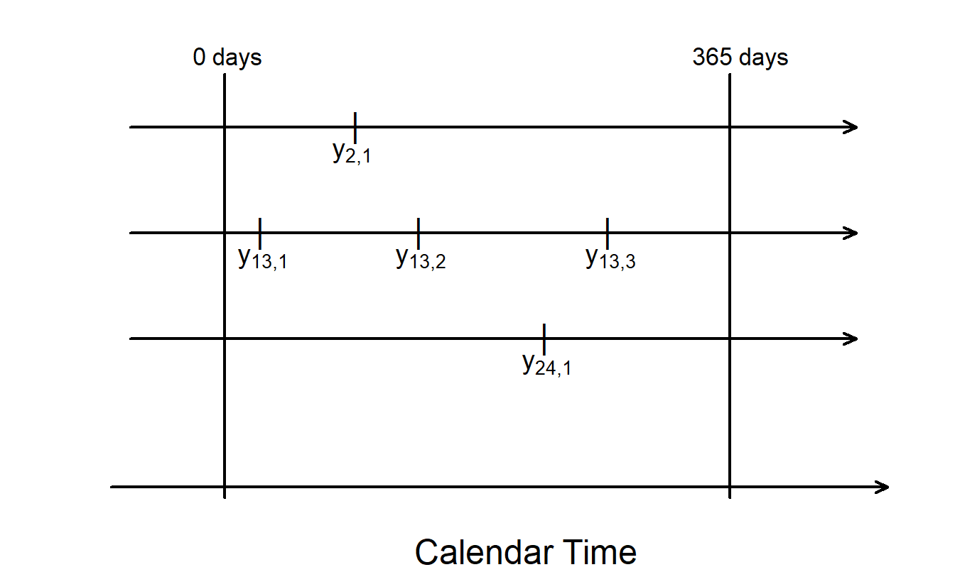
Figure 14.5: Figure Illustrating (Potentially) Repeated Warranty Claims.
We present models of recurrent events using counting processes, specifically employ Poisson processes. Although there are alternative approaches, for statistical analyses the counting process concept seems the most fruitful (Cook and Lawless, 2007). Moreover, there is a strong historical connection of Poisson processes with actuarial ruin theory (Klugman, Panjer and Willmot, 2008, Chapter 11) and so many actuaries are familiar with Poisson processes.
Let \(N_i(t)\) be the number of events that have occurred by time \(t\). Using algebra, we can write this as \(N_i(t) = \sum_{j \geq 1} \mathrm{I}(y_{ij} \leq t).\) Because \(N_i(t)\) varies with a subject’s experience, it is a random variable for each fixed \(t\). Further, when viewing the entire evolution of claims, \(\{N_i(t), t \geq 0 \}\), is known as a stochastic process. A counting process is a special kind of stochastic process that describes counts that are monotonically increasing over time. A Poisson process is a special kind of counting process. If \(\{N_i(t), t \geq 0 \}\) is a Poisson process, then \(N_i(t)\) has a Poisson distribution with mean, say, \(\mathrm{h}_i(t)\) for each fixed \(t\). In the counting process literature, it is customary to refer to \(\mathrm{h}_i(t)\) as the intensity function.
Statistical inference for recurrent events can be conducted using Poisson processes and parametric maximum likelihood techniques. As discussed in Cook and Lawless (2007), the likelihood for the \(i\)th subject is based on the conditional probability density of the observed outcomes “\(m_i\) events, at times \(y_{i1} < \cdots < y_{im_i}\)”. This yields the likelihood \[\begin{equation} Likelihood_i = \prod_{j=1}^{m_i} \{\mathrm{h}_i(y_{ij}) \} \exp \left(- \int_0^{\infty} y_i(s) \mathrm{h}_i(s) ds \right) \tag{14.5} \end{equation}\] where \(y_i(s)\) is a binary variable to indicate whether the \(i\)th subject is observed by time \(s\).
To parameterize the intensity function \(\mathrm{h}_i(t)\), we assume that we have available explanatory variables. For example, when examining warranty automobile claims, we might have available the make and model of the vehicle, or driver characteristics such as gender and age at time of purchase. We might have characteristics that are functions of the time of claim, such as the number of miles driven. Thus, we use the notation \(\mathbf{x}_i(t)\) to denote the potential dependence of the explanatory variables on the event time.
Similar to equation (14.3), it is customary to write the intensity function as \[ h_i(t) = h_0(t) \exp( \mathbf{x}_i^{\prime}(t) \boldsymbol \beta ). \] where \(h_0(t)\) is the baseline intensity. For a full parametric specification, one would specify the baseline intensity in terms of several parameters. Then, one would use the intensity function \(h_i(t)\) in the likelihood equation (14.5) that would serve as the basis for likelihood inference. As discussed in Cook and Lawless (2007), semi-parametric approaches where the baseline is not fully parametrically specified (such as the \(PH\) model) are also possible.
14.6 Further Reading and References
As described in Collett (1994), the product-limit estimator had been used since the early part of the twentieth century. Greenwood (1926) established the formula for an approximate variance. The work of Kaplan and Meier (1958) is often associated with the product-limit estimator; they showed that it is a nonparametric maximum likelihood estimator of the survival function.
There are several good sources for further study of survival analysis, particularly in the biomedical sciences; Collett (1994) is a one such source. The text by Klein and Moeschberger (1997) was used for several years as required reading for the North American Society of Actuaries syllabus. Lawless (2003) provides an introduction from an engineering perspective. Lancaster (1990) discusses econometric issues. Hougaard (2000) provides an advanced treatment.
We refer to Cook and Lawless (2007) for a book-long treatment of recurrent events.
Chapter References
- Breslow, Norman (1974). Covariance analysis of censored survival data. Biometrics 30, 89-99.
- Collett, D. (1994). Modelling Survival Data in Medical Research. Chapman & Hall, London.
- Cook, Richard J. and Jerald F. Lawless (2007). The Statistical Analysis of Recurrent Events. Springer-Verlag, New York.
- Cox, David R. (1972). Regression models and life-tables. Journal of the Royalty Statistical Society, Series B 34, 187-202.
- Gourieroux, Christian and Joann Jasiak (2007). The Econometrics of Individual Risk. Princeton University Press, Princeton, New Jersey.
- Greenwood, M. (1926). The errors of sampling of the survivorship tables. Reports on Public Health and Statistical Subjects, number 33, Appendix, HMSO, London.
- Kaplan, E. L. and Meier, P. (1958). Nonparametric estimation from incomplete observations. Journal of the American Statistical Association 53, 457-481.
- Kim, Yong-Duck, Dan R. Anderson, Terry L. Amburgey and James C. Hickman (1995). The use of event history analysis to examine insurance insolvencies. Journal of Risk and Insurance 62, 94-110.
- Klein, John P. and Melvin L. Moeschberger (1997). Survival Analysis: Techniques for Censored and Truncated Data. Springer-Verlag, New York.
- Klugman, Stuart A, Harry H. Panjer and Gordon E. Willmot (2008). Loss Models: From Data to Decisions. John Wiley & Sons, Hoboken, New Jersey.
- Lancaster, Tony (1990). The Econometric Analysis of Transition Data. Cambridge University Press, New York.
- Lawless, Jerald F. (2003). Statistical Models and Methods for Lifetime Data, Second Edition. John Wiley & Sons, New York.
- Hougaard, Philip (2000). Analysis of Multivariate Survival Data. Springer-Verlag, New York.
- Miller, Rupert G. (1997). Survival Analysis. John Wiley & Sons, New York.
- Shumway, Tyler (2001). Forecasting bankruptcy more accurately: A simple hazard model. Journal of Business 74, 101-124.
- Stepanova, Maria and Lyn Thomas (2002). Survival analysis methods for personal loan data. Operations Research 50(2), 277-290.
- Zhou, Mai (2001). Understanding the Cox regression models with time-changing covariates. American Statistician 55(2), 153-155.