Chapter 11 Categorical Dependent Variables
Chapter Preview. A model with a categorical dependent variable allows one to predict whether an observation is a member of a distinct group, or category. Binary variables represent an important special case; they can indicate whether or not an event of interest has occurred. In actuarial and financial applications, the event may be whether a claim occurs, a person purchases insurance, a person retires or a firm becomes insolvent. The chapter introduces logistic regression and probit models of binary dependent variables. Categorical variables may also represent more than two groups, known as multicategory outcomes. Multicategory variables may be unordered or ordered, depending on whether it makes sense to rank the variable outcomes. For unordered outcomes, known as nominal variables, the chapter introduces generalized logits and multinomial logit models. For ordered outcomes, known as ordinal variables, the chapter introduces cumulative logit and probit models.
11.1 Binary Dependent Variables
We have already introduced binary variables as a special type of discrete variable that can be used to indicate whether or not a subject has a characteristic of interest, such as sex for a person or ownership of a captive insurance company for a firm. Binary variables also describe whether or not an event of interest has occurred, such as an accident. A model with a binary dependent variable allows one to predict whether an event has occurred or a subject has a characteristic of interest.
Example: MEPS Expenditures. Section 11.4 will describe an extensive database from the Medical Expenditure Panel Survey (MEPS) on hospitalization utilization and expenditures. For these data, we will consider \[ y_i = \left\{ \begin{array}{ll} 1 & \text{i-th person was hospitalized during the sample period} \\ 0 & \text{otherwise} \end{array} \right. . \] There are \(n=2,000\) persons in this sample, distributed as:
| Male | Female | ||
|---|---|---|---|
| Not hospitalized | \(y=0\) | 902 (95.3%) | 941 (89.3%) |
| Hospitalized | \(y=1\) | 44 (4.7%) | 113 (10.7%) |
| Total | 946 | 1,054 |
R Code to Produce Table 11.1
Table 11.1 suggests that sex has an important influence on whether someone becomes hospitalized.
Like the linear regression techniques introduced in prior chapters, we are interested in using characteristics of a person, such as their age, sex, education, income and prior health status, to help explain the dependent variable \(y\). Unlike the prior chapters, now the dependent variable is discrete and not even approximately normally distributed. In limited circumstances, linear regression can be used with binary dependent variables — this application is known as a linear probability model.
Linear probability models
To introduce some of the complexities encountered with binary dependent variables, denote the probability that the response equals 1 by \(\pi_i= \mathrm{Pr}(y_i=1)\). A binary random variable has a Bernoulli distribution. Thus, we may interpret the mean response as the probability that the response equals one, that is, \(\mathrm{E~}y_i=0\times \mathrm{Pr}(y_i=0) + 1 \times \mathrm{Pr}(y_i=1) = \pi_i\). Further, the variance is related to the mean through the expression \(\mathrm{Var}~y_i = \pi_i(1-\pi_i)\).
We begin by considering a linear model of the form \[ y_i = \mathbf{x}_i^{\mathbf{\prime}} \boldsymbol \beta + \varepsilon_i, \]
known as a linear probability model. Assuming \(\mathrm{E~}\varepsilon_i=0\), we have that \(\mathrm{E~}y_i=\mathbf{x}_i^{\mathbf{\prime }} \boldsymbol \beta =\pi_i\). Because \(y_i\) has a Bernoulli distribution, \(\mathrm{Var}~y_i=\mathbf{x}_i^{\mathbf{\prime}} \boldsymbol \beta(1-\mathbf{x}_i^{\mathbf{\prime}}\boldsymbol \beta)\). Linear probability models are used because of the ease of parameter interpretations. For large data sets, the computational simplicity of ordinary least squares estimators is attractive when compared to some complex alternative nonlinear models introduced later in this chapter. As described in Chapter 3, ordinary least squares estimators for \(\boldsymbol \beta\) have desirable properties. It is straightforward to check that the estimators are consistent and asymptotically normal under mild conditions on the explanatory variables {\(\mathbf{x}_i\)}. However, linear probability models have several drawbacks that are serious for many applications.
Drawbacks of the Linear Probability Model
Fitted values can be poor. The expected response is a probability and thus must vary between 0 and 1. However, the linear combination, \(\mathbf{x}_i^{\mathbf{\prime}} \boldsymbol \beta\), can vary between negative and positive infinity. This mismatch implies, for example, that fitted values may be unreasonable.
Heteroscedasticity. Linear models assume homoscedasticity (constant variance), yet the variance of the response depends on the mean that varies over observations. The problem of varying variability is known as heteroscedasticity.
Residual analysis is meaningless. The response must be either a 0 or 1 although the regression models typically regard the distribution of the error term as continuous. This mismatch implies, for example, that the usual residual analysis in regression modeling is meaningless.
To handle the heteroscedasticity problem, a (two-stage) weighted least squares procedure is possible. In the first stage, one uses ordinary least squares to compute estimates of \(\boldsymbol \beta\). With this estimate, an estimated variance for each subject can be computed using the relation \(\mathrm{Var}~y_i=\mathbf{x}_i^{\mathbf{\prime}}\boldsymbol \beta (1-\mathbf{x}_i^{\mathbf{\prime}}\boldsymbol \beta)\). At the second stage, a weighted least squares is performed using the inverse of the estimated variances as weights to arrive at new estimates of \(\boldsymbol \beta\). It is possible to iterate this procedure, although studies have shown that there are few advantages in doing so (see Carroll and Ruppert, 1988). Alternatively, one can use ordinary least squares estimators of \(\boldsymbol \beta\) with standard errors that are robust to heteroscedasticity (see Section 5.7.2).
Video: Section Summary
11.2 Logistic and Probit Regression Models
11.2.1 Using Nonlinear Functions of Explanatory Variables
To circumvent the drawbacks of linear probability models, we consider alternative models in which we express the expectation of the response as a function of explanatory variables, \(\pi_i=\mathrm{\pi }(\mathbf{x}_i^{\mathbf{\prime}}\boldsymbol \beta)\) \(=\Pr (y_i=1|\mathbf{x}_i)\). We focus on two special cases of the function \(\mathrm{\pi }(\cdot)\):
\(\mathrm{\pi }(z)=\frac{1}{1+\exp (-z)}=\frac{e^{z}}{1+e^{z}}\), the logit case, and
\(\mathrm{\pi }(z)=\mathrm{\Phi }(z)\), the probit case.
Here, \(\mathrm{\Phi }(\cdot)\) is the standard normal distribution function. The choice of the identity function (a special kind of linear function), \(\mathrm{\pi }(z)=z\), yields the linear probability model. In contrast, \(\mathrm{\pi}\) is nonlinear for both the logit and probit cases. These two functions are similar in that they are almost linearly related over the interval \(0.1 \le p \le 0.9\). Thus, to a large extent, the function choice is dependent on the preferences of the analyst. Figure 11.1 compares the logit and probit functions showing that it will be difficult to distinguish between the two specifications with most data sets.
The inverse of the function, \(\mathrm{\pi }^{-1}\), specifies the form of the probability that is linear in the explanatory variables, that is, \(\mathrm{\pi }^{-1}(\pi_i)= \mathbf{x}_i^{\mathbf{\prime}}\boldsymbol \beta\). In Chapter 13, we refer to this inverse as the link function.
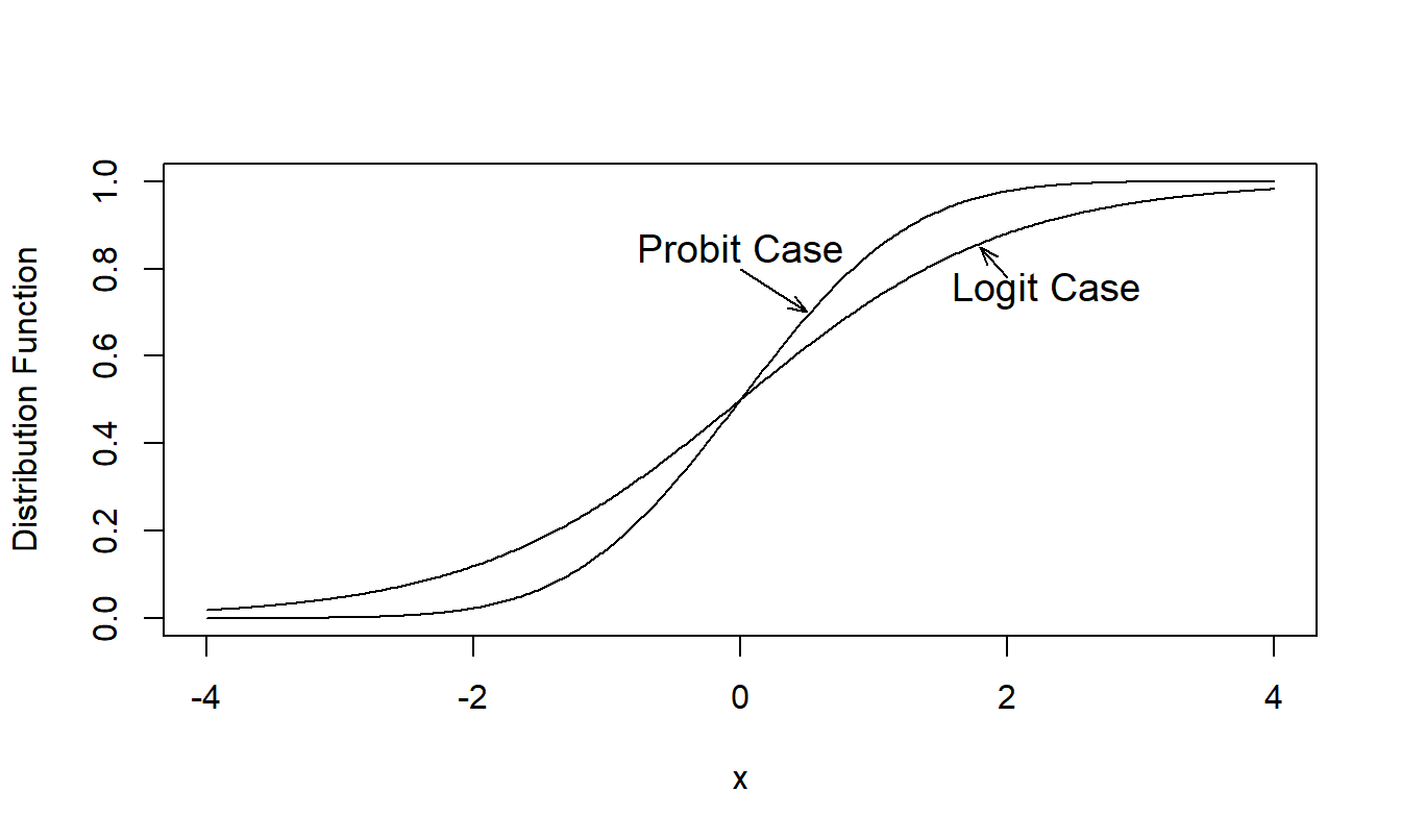
Figure 11.1: Comparison of Logit and Probit (Standard Normal) Distribution
Example: Credit Scoring. Banks, credit bureaus, and other financial institutions develop “credit scores” for individuals that are used to predict the likelihood that the borrower will repay current and future debts. Individuals who do not meet stipulated repayment schedules in a loan agreement are said to be in “default.” A credit score is then a predicted probability of being in default, with the credit application providing the explanatory variables used in developing the credit score. The choice of explanatory variables depends on the purpose of the application; credit scoring is used for issuing credit cards for making small consumer purchases as well as mortgage applications for multimillion dollar houses. In Table 11.2, Hand and Henley (1997) provide a list of typical characteristics that are used in credit scoring.
Table 11.2. Characteristics Used in Some Credit Scoring Procedures
\[ \small{ \begin{array}{ll} \hline \textbf{Characteristics} & \textbf{Potential Values} \\ \hline \text{Time at present address} & \text{0-1, 1-2, 3-4, 5+ years}\\ \text{Home status} & \text{Owner, tenant, other }\\ \text{Postal Code} & \text{Band A, B, C, D, E} \\ \text{Telephone} & \text{Yes, no} \\ \text{Applicant's annual income} & \text{£ (0-10000),} \text{£ (10,000-20,000)} \text{£ (20,000+)} \\ \text{Credit card} & \text{Yes, no} \\ \text{Type of bank account} & \text{Check and/or savings, none} \\ \text{Age }& \text{18-25, 26-40, 41-55, 55+ years} \\ \text{County Court judgements} & \text{Number} \\ \text{Type of occupation} & \text{Coded} \\ \text{Purpose of loan} & \text{Coded} \\ \text{Marital status} & \text{Married, divorced, single, widow, other} \\ \text{Time with bank} & \text{Years} \\ \text{Time with employer} & \text{Years }\\ \hline \textit{Source}: \text{Hand and Henley (1997)} \\ \end{array} } \]
With credit application information and default experience, a logistic regression model can be used to fit the probability of default with credit scores resulting from fitted values. Wiginton (1980) provides an early application of logistic regression to consumer credit scoring. At that time, other statistical methods known as discriminant analysis were at the cutting edge of quantitative scoring methodologies. In their review article, Hand and Henley (1997) discuss other competitors to logistic regression including machine learning systems and neural networks. As noted by Hand and Henley, there is no uniformly “best” method. Regression techniques are important in their own right due to their widespread usage and because they can provide a platform for learning about newer methods.
Credit scores provide estimates of the likelihood of defaulting on loans but issuers of credit are also interested in the amount and timing of debt repayment. For example, a “good” risk may repay a credit balance so promptly that little profit is earned by the lender. Further, a “poor” mortgage risk may default on a loan so late in the duration of the contract that a sufficient profit was earned by the lender. See Gourieroux and Jasiak (2007) for a broad discussion of how credit modeling can be used to assess the riskiness and profitability of loans.
11.2.2 Threshold Interpretation
Both the logit and probit cases can be interpreted as follows. Suppose that there exists an underlying linear model, \(y_i^{\ast} = \mathbf{x}_i^{\mathbf{\prime}}\boldsymbol \beta + \varepsilon_i^{\ast}\). Here, we do not observe the response \(y_i^{\ast}\) yet interpret it to be the “propensity” to possess a characteristic. For example, we might think about the financial strength of an insurance company as a measure of its propensity to become insolvent (no longer capable of meeting its financial obligations). Under the threshold interpretation, we do not observe the propensity but we do observe when the propensity crosses a threshold. It is customary to assume that this threshold is 0, for simplicity. Thus, we observe \[ y_i=\left\{ \begin{array}{ll} 0 & y_i^{\ast} \le 0 \\ 1 & y_i^{\ast}>0 \end{array} \right. . \] To see how the logit case is derived from the threshold model, assume a logistic distribution function for the disturbances, so that \[ \mathrm{\Pr }(\varepsilon_i^{\ast} \le a)=\frac{1}{1+\exp (-a)}. \] Like the normal distribution, one can verify by calculating the density that the logistic distribution is symmetric about zero. Thus, \(-\varepsilon_i^{\ast}\) has the same distribution as \(\varepsilon_i^{\ast}\) and so \[ \pi_i=\Pr (y_i=1|\mathbf{x}_i)=\mathrm{\Pr }(y_i^{\ast}>0)=\mathrm{ \Pr }(\varepsilon_i^{\ast} \le \mathbf{x}_i^{\mathbf{\prime}}\mathbf{ \beta })=\frac{1}{1+\exp (-\mathbf{x}_i^{\mathbf{\prime}}\boldsymbol \beta)} =\mathrm{\pi }(\mathbf{x}_i^{\mathbf{\prime}}\boldsymbol \beta). \] This establishes the threshold interpretation for the logit case. The development for the probit case is similar and is omitted.
11.2.3 Random Utility Interpretation
Both the logit and probit cases are also justified by appealing to the following “random utility” interpretation of the model. In some economic applications, individuals select one of two choices. Here, preferences among choices are indexed by an unobserved utility function; individuals select the choice that provides the greater utility.
For the \(i\)th subject, we use the notation \(u_i\) for this utility function. We model the utility (\(U\)) as a function of an underlying value (\(V\)) plus random noise (\(\varepsilon\)), that is, \(U_{ij}=u_i(V_{ij}+\varepsilon_{ij})\), where \(j\) may be 1 or 2, corresponding to the choice. To illustrate, we assume that the individual chooses the category corresponding to \(j=1\) if \(U_{i1}>U_{i2}\) and denote this choice as \(y_i=1\). Assuming that \(u_i\) is a strictly increasing function, we have \[\begin{eqnarray*} \Pr (y_i &=&1)=\mathrm{\Pr }(U_{i2}<U_{i1})=\mathrm{\Pr }\left( u_i(V_{i2}+\varepsilon_{i2})<u_i(V_{i1}+\varepsilon_{i1})\right) \\ &=&\mathrm{\Pr }(\varepsilon_{i2}-\varepsilon_{i1}<V_{i1}-V_{i2}). \end{eqnarray*}\]
To parameterize the problem, assume that the value \(V\) is an unknown linear combination of explanatory variables. Specifically, we take \(V_{i2}=0\) and \(V_{i1}=\mathbf{x}_i^{\mathbf{\prime}}\boldsymbol \beta\). We may take the difference in the errors, \(\varepsilon_{i2}-\varepsilon_{i1}\), as normal or logistic, corresponding to the probit and logit cases, respectively. The logistic distribution is satisfied if the errors are assumed to have an extreme-value, or Gumbel, distribution (see, for example, Amemiya, 1985).
Video: Section Summary
11.2.4 Logistic Regression
An advantage of the logit case is that it permits closed-form expressions, unlike the normal distribution function. Logistic regression is another phrase used to describe the logit case.
Using \(p=\mathrm{\pi }(z)= \left( 1+ \mathrm{e}^{-z}\right)^{-1}\), the inverse of \(\mathrm{\pi }\) is calculated as \(z=\mathrm{\pi }^{-1}(p)=\ln(p/(1-p))\). To simplify future presentations, we define \[ \mathrm{logit}(p)=\ln \left( \frac{p}{1-p}\right) \] to be the logit function. With a logistic regression model, we represent the linear combination of explanatory variables as the logit of the success probability, that is, \(\mathbf{x}_i^{\mathbf{\prime}}\boldsymbol \beta=\mathrm{logit}(\pi_i)\).
Odds interpretation
When the response \(y\) is binary, knowing only \(p=\Pr(y=1)\) summarizes the entire distribution. In some applications, a simple transformation of \(p\) has an important interpretation. The lead example of this is the odds, given by \(p/(1-p)\). For example, suppose that \(y\) indicates whether or not a horse wins a race and \(p\) is the probability of the horse winning. If \(p=0.25\), then the odds of the horse winning is $ 0.25/(1.00-0.25)=0.3333$. We might say that the odds of winning are 0.3333 to 1, or one to three. Equivalently, we say that the probability of not winning is \(1-p=0.75\) so that the odds of the horse not winning is $ 0.75/(1-0.75)=3$ and the odds against the horse are three to one.
Odds have a useful interpretation from a betting standpoint. Suppose that we are playing a fair game and that we place a bet of 1 with one to three odds. If the horse wins, then we get our 1 back plus winnings of 3. If the horse loses, then we lose our bet of 1. It is a fair game in the sense that the expected value of the game is zero because we win 3 with probability \(p=0.25\) and lose 1 with probability \(1-p=0.75\). From an economic standpoint, the odds provide the important numbers (bet of 1 and winnings of 3), not the probabilities. Of course, if we know \(p\), then we can always calculate the odds. Similarly, if we know the odds, we can always calculate the probability \(p\).
The logit is the logarithmic odds function, also known as the log odds.
Odds ratio interpretation
To interpret the regression coefficients in the logistic regression model, \(\boldsymbol \beta=(\beta_0,\ldots ,\beta_{k})^{\prime}\), we begin by assuming that \(j\)th explanatory variable, \(x_{ij}\), is either 0 or 1. Then, with the notation \(\mathbf{x}_i=(x_{i0},...,x_{ij},\ldots ,x_{ik})^{\prime}\), we may interpret
\[\begin{eqnarray*} \beta_j &=&(x_{i0},...,1,\ldots ,x_{ik})^{\prime}\boldsymbol \beta -(x_{i0},...,0,\ldots ,x_{ik})^{\prime}\boldsymbol \beta \\ &=&\ln \left( \frac{\Pr (y_i=1|x_{ij}=1)}{1-\Pr (y_i=1|x_{ij}=1)}\right) -\ln \left( \frac{\Pr (y_i=1|x_{ij}=0)}{1-\Pr (y_i=1|x_{ij}=0)}\right) \end{eqnarray*}\]
Thus,
\[ e^{\beta_j}=\frac{\Pr (y_i=1|x_{ij}=1)/\left( 1-\Pr (y_i=1|x_{ij}=1)\right) }{\Pr (y_i=1|x_{ij}=0)/\left( 1-\Pr (y_i=1|x_{ij}=0)\right) }. \] This shows that \(e^{\beta_j}\) can be expressed as the ratio of two odds, known as the odds ratio. That is, the numerator of this expression is the odds when \(x_{ij}=1,\) whereas the denominator is the odds when \(x_{ij}=0\). Thus, we can say that the odds when \(x_{ij}=1\) are \(\exp (\beta_j)\) times as large as the odds when \(x_{ij}=0\). To illustrate, suppose \(\beta_j=0.693\), so that \(\exp (\beta _j)=2\). From this, we say that the odds (for \(y=1\)) are twice as great for \(x_{ij}=1\) as for \(x_{ij}=0\).
Similarly, assuming that \(j\)th explanatory variable is continuous (differentiable), we have \[\begin{eqnarray} \beta_j &=&\frac{\partial }{\partial x_{ij}}\mathbf{x}_i^{\prime} \boldsymbol \beta =\frac{\partial }{\partial x_{ij}}\ln \left( \frac{\Pr (y_i=1|x_{ij})}{1-\Pr (y_i=1|x_{ij})}\right) \nonumber \\ &=&\frac{\frac{\partial }{\partial x_{ij}}\Pr (y_i=1|x_{ij})/\left( 1-\Pr (y_i=1|x_{ij})\right) }{\Pr (y_i=1|x_{ij})/\left( 1-\Pr (y_i=1|x_{ij})\right) }. \tag{11.1} \end{eqnarray}\] Thus, we may interpret \(\beta_j\) as the proportional change in the odds ratio, known as an elasticity in economics.
Example: MEPS Expenditures - Continued. Table 11.1 shows that the percentage of females who were hospitalized is \(10.7\%\); alternatively, the odds of females being hospitalized is \(0.107/(1-0.107)=0.120\). For males, the percentage is \(4.7\%\) so that the odds were \(0.0493\). The odds ratio is \(0.120/0.0493=2.434\); females are more than twice as likely to be hospitalized as males.
From a logistic regression fit (described in Section 11.4), the coefficient associated with sex is \(0.733\). Based on this model, we say that females are \(\exp (0.733)=2.081\) times as likely as males to be hospitalized. The regression estimate of the odds ratio controls for additional variables (such as age and education) compared to the basic calculation based on raw frequencies.
Video: Section Summary
11.3 Inference for Logistic and Probit Regression Models
11.3.1 Parameter Estimation
The customary method of estimation for logistic and probit models is maximum likelihood, described in further detail in Section 11.9. To provide intuition, we outline the ideas in the context of binary dependent variable regression models.
The likelihood is the observed value of the probability function. For a single observation, the likelihood is \[ \left\{ \begin{array}{ll} 1-\pi_i & \mathrm{if}\ y_i=0 \\ \pi_i & \mathrm{if}\ y_i=1 \end{array} \right. . \] The objective of maximum likelihood estimation is to find the parameter values that produce the largest likelihood. Finding the maximum of the logarithmic function yields the same solution as finding the maximum of the corresponding function. Because it is generally computationally simpler, we consider the logarithmic (or log-) likelihood, written as \[\begin{equation} \left\{ \begin{array}{ll} \ln \left( 1-\pi_i\right) & \mathrm{if}\ y_i=0 \\ \ln \pi_i & \mathrm{if}\ y_i=1 \end{array} \right. . \tag{11.2} \end{equation}\] More compactly, the log-likelihood of a single observation is \[ y_i\ln \mathrm{\pi }(\mathbf{x}_i^{\mathbf{\prime}}\boldsymbol \beta) + (1-y_i) \ln \left( 1-\mathrm{\pi }(\mathbf{x}_i^{\mathbf{\prime}} \boldsymbol \beta)\right) , \] where \(\pi_i=\mathrm{\pi }(\mathbf{x}_i^{\mathbf{\prime}}\boldsymbol \beta )\). Assuming independence among observations, the likelihood of the data set is a product of likelihoods of each observation. Taking logarithms, the log-likelihood of the data set is the sum of log-likelihoods of single observations.
The log-likelihood of the data set is \[\begin{equation} L(\boldsymbol \beta)=\sum\limits_{i=1}^{n}\left\{ y_i\ln \mathrm{\pi }( \mathbf{x}_i^{\mathbf{\prime}}\boldsymbol \beta) + (1-y_i) \ln \left( 1- \mathrm{\pi }(\mathbf{x}_i^{\mathbf{\prime}}\boldsymbol \beta)\right) \right\} . \tag{11.3} \end{equation}\] The log-likelihood is viewed as a function of the parameters, with the data held fixed. In contrast, the joint probability mass function is viewed as a function of the realized data, with the parameters held fixed.
The method of maximum likelihood involves finding the values of \(\boldsymbol \beta\) that maximize the log-likelihood. The customary method of finding the maximum is taking partial derivatives with respect to the parameters of interest and finding roots of the resulting equations. In this case, taking partial derivatives with respect to \(\boldsymbol \beta\) yields the score equations
\[\begin{equation} \frac{\partial }{\partial \boldsymbol \beta}L(\boldsymbol \beta )=\sum\limits_{i=1}^{n}\mathbf{x}_i\left( y_i-\mathrm{\pi }(\mathbf{x}_i^{\mathbf{\prime}}\boldsymbol \beta)\right) \frac{\mathrm{\pi }^{\prime}( \mathbf{x}_i^{\mathbf{\prime}}\boldsymbol \beta)}{\mathrm{\pi }(\mathbf{x}_i^{\mathbf{\prime}}\boldsymbol \beta)(1-\mathrm{\pi }(\mathbf{x}_i^{ \mathbf{\prime}}\boldsymbol \beta))}=\mathbf{0}, \tag{11.4} \end{equation}\] where \(\pi^{\prime}\) is the derivative of \(\pi\). The solution of these equations, denoted as \(\mathbf{b}_{MLE}\), is the maximum likelihood estimator. For the logit function the score equations reduce to
\[\begin{equation} \frac{\partial }{\partial \boldsymbol \beta}L(\boldsymbol \beta )=\sum\limits_{i=1}^{n}\mathbf{x}_i\left( y_i-\mathrm{\pi }(\mathbf{x} _i^{\mathbf{\prime}}\boldsymbol \beta)\right) =\mathbf{0}, \tag{11.5} \end{equation}\] where \(\mathrm{\pi }(z)=1/(1+\exp (-z))\).
11.3.2 Additional Inference
An estimator of the large sample variance of \(\boldsymbol \beta\) may be calculated taking partial derivatives of the score equations. Specifically, the term \[ \mathbf{I}(\boldsymbol \beta) = - \mathrm{E} \left( \frac{\partial^2} {\partial \boldsymbol \beta ~ \partial \boldsymbol \beta ^{\prime}}L(\boldsymbol \beta) \right) \] is the information matrix. As a special case, using the logit function and equation (11.5), straightforward calculations show that the information matrix is \[ \mathbf{I}(\boldsymbol \beta) = \sum\limits_{i=1}^{n} \sigma_i^2 \mathbf{x}_i \mathbf{x}_i^{\prime} \] where \(\sigma_i^2 = \mathrm{\pi} (\mathbf{x}_i^{\prime} \boldsymbol \beta) (1 - \mathrm{\pi}(\mathbf{x}_i^{\prime} \boldsymbol \beta))\). The square root of the \((j+1)st\) diagonal element of this matrix evaluated at \(\boldsymbol \beta = \mathbf{b}_{MLE}\) yields the standard error for \(b_{j,MLE}\), denoted as \(se(b_{j,MLE})\).
To assess the overall model fit, it is customary to cite likelihood ratio test statistics in nonlinear regression models. To test the overall model adequacy \(H_0:\boldsymbol \beta=\mathbf{0}\), we use the statistic \[ LRT=2\times (L(\mathbf{b}_{MLE})-L_0), \] where \(L_0\) is the maximized log-likelihood with only an intercept term. Under the null hypothesis \(H_0\), this statistic has a chi-square distribution with \(k\) degrees of freedom. Section 11.9.3 describes likelihood ratio test statistics in greater technical detail.
As described in Section 11.9, measures of goodness of fit can be difficult to interpret in nonlinear models. One measure is the so-called \(max-scaled~R^2\), defined as \(R_{ms}^2=R^2/R_{max}^2\), where \[ R^2=1-\left( \frac{\exp (L_0/n)}{\exp (L(\mathbf{b}_{MLE})/n)}\right) \] and \(R_{max }^2 = 1 - \exp(L_0/n)^2\). Here, \(L_0/n\) represents the average value of this log-likelihood.
Another measure is a “pseudo-\(R^2\)” \[ \frac{L( \mathbf{b}_{MLE}) - L_0}{L_{max}-L_0}, \] where \(L_0\) and \(L_{max }\) is the log-likelihood based on only an intercept and on the maximum achievable, respectively. Like the coefficient of determination, the pseudo-\(R^2\) takes on values between zero and one, with larger values indicating a better fit to the data. Other versions of pseudo-\(R^2\)’s are available in the literature, see, for example, Cameron and Trivedi (1998). An advantage of this pseudo-\(R^2\) measure is its link to hypothesis testing of regression coefficients.
Example: Job Security. Valletta (1999) studied declining job security using the Panel Survey of Income Dynamics (PSID) database. We consider here one of the regression models presented by Valletta, based on a sample of male heads of households that consists of \(n=24,168\) observations over the years 1976-1992, inclusive. The PSID survey records reasons why men left their most recent employment, including plant closures, “quit”and changed jobs for other reasons. However, Valletta focused on dismissals (“laid off” or “fired”) because involuntary separations are associated with job insecurity.
Table 11.3 presents a probit regression model run by Valletta (1999), using dismissals as the dependent variable. In addition to the explanatory variables listed in Table 11.3, other variables controlled for consisted of education, marital status, number of children, race, years of full-time work experience and its square, union membership, government employment, logarithmic wage, the U.S. employment rate and location as measured through the Metropolitan Statistical Area residence. In Table 11.3, tenure is years employed at the current firm. Further, sector employment was measured by examining the Consumer Price Survey employment in 387 sectors of the economy, based on 43 industry categories and nine regions of the country.
On the one hand, the tenure coefficient reveals that more experienced workers are less likely to be dismissed. On the other hand, the coefficient associated with the interaction between tenure and time trend reveals an increasing dismissal rate for experienced workers.
The interpretation of the sector employment coefficients is also of interest. With an average tenure of about 7.8 years in the sample, we see the low tenure men are relatively unaffected by changes in sector employment. However, for more experienced men, there is an increasing probability of dismissal associated with sectors of the economy where growth declines.
Table 11.3. Dismissal Probit Regression Estimates
\[ \small{ \begin{array}{lrr} \hline \textbf{Variable} & \textbf{Parameter} & \textbf{Standard} \\ & \textbf{Estimate} & \textbf{Error} \\ \hline \text{Tenure} & -0.084 & 0.010 \\ \text{Time Trend} & -0.002 & 0.005 \\ \text{Tenure*(Time Trend)} & 0.003 & 0.001 \\ \text{Change in Logarithmic Sector Employment} & 0.094 & 0.057 \\ \text{Tenure*( Change in Logarithmic Sector Employment)} & -0.020 & 0.009 \\ \hline \text{-2 Log Likelihood }& 7,027.8 & \\ \text{Pseudo}-R^2 & 0.097 & \\ \hline \end{array} } \]
Video: Section Summary
11.4 Application: Medical Expenditures
This section considers data from the Medical Expenditure Panel Survey (MEPS), conducted by the U.S. Agency of Health Research and Quality. MEPS is a probability survey that provides nationally representative estimates of health care use, expenditures, sources of payment, and insurance coverage for the U.S. civilian population. This survey collects detailed information on individuals and each medical care episode by type of services including physician office visits, hospital emergency room visits, hospital outpatient visits, hospital inpatient stays, all other medical provider visits, and use of prescribed medicines. This detailed information allows one to develop models of health care utilization to predict future expenditures. We consider MEPS data from the first panel of 2003 and take a random sample of \(n=2,000\) individuals between ages 18 and 65.
Dependent Variable
Our dependent variable is an indicator of positive expenditures for inpatient admissions. For MEPS, inpatient admissions include persons who were admitted to a hospital and stayed overnight. In contrast, outpatient events include hospital outpatient department visits, office-based provider visits and emergency room visits excluding dental services. (Dental services, compared to other types of health care services, are more predictable and occur on a more regular basis.) Hospital stays with the same date of admission and discharge, known as “zero-night stays,” were included in outpatient counts and expenditures. Payments associated with emergency room visits that immediately preceded an inpatient stay were included in the inpatient expenditures. Prescribed medicines that can be linked to hospital admissions were included in inpatient expenditures (not in outpatient utilization).
Explanatory Variables
Explanatory variables that can help explain health care utilization are categorized as demographic, geographic, health status, education and economic factors. Demographic factors include age, sex and ethnicity. As persons age, the rate at which their health deteriorates increases with age; as a result, age has an increasing impact on the demand for health care. Sex and ethnicity can be treated as proxies for inherited health and social habits in maintaining health. For a geographic factor, we use region to proxy the accessibility of health care services and the overall economic or regional impact on residents’ health care behavior.
The demand for medical services is thought to be influenced by individuals’ health status and education. In MEPS, self-rated physical health, mental health and any functional or activity related limitations during the sample period are used as proxies for health status. Education tends to have ambiguous impact on the demand for health care services. One theory is that more educated persons are more aware of health risks, thus being more active in maintaining their health; as a result, educated persons may be less prone to severe diseases leading to hospital admissions. Another theory is that less educated persons have greater exposure to health risks and, through exposure, develop a greater tolerance for certain types of risks. In MEPS, education is proxied by degrees received and categorized into three different levels: lower than high school, high school, and college or above education.
Economic covariates include income and insurance coverage. A measure of income in MEPS is income relative to the poverty line. This approach is appropriate because it summarizes effects of different levels of income on health care utilization in constant dollars. Insurance coverage is also an important variable in explaining health care utilization. One issue with health insurance coverage is that it reduces the out-of-pocket prices paid by insureds and thus induces moral hazard. Research associated with the Rand Health Insurance Experiment empirically suggested that cost sharing effects from insurance coverage will affect primarily the number of medical contacts rather than the intensity of each contact. This motivated our introduction of a binary variable that takes the value of 1 if a person had any public or private health insurance for at least one month, and 0 otherwise.
Summary Statistics
Table 11.4 describes these explanatory variables and provides summary statistics that suggest their effects on the probability of positive inpatient expenditures. For example, we see that females had a higher overall utilization than males. Specifically, 10.7% of females had a positive expenditure during the year compared to only 4.7% for males. Similarly, utilizations vary by other covariates, suggesting their importance as predictors of expenditures.
Table 11.4. Percent of Positive Expenditures by Explanatory Variable
\[ \scriptsize{ \begin{array}{lllrr} \hline \textbf{Category} & \textbf{Variable} & \textbf{Description} & \textbf{Percent} & \textbf{Percent} \\ & & & \textbf{of data} & \textbf{Positive} \\ & & & & \textbf{Expend} \\ \hline \text{Demography} & AGE & \text{Age in years between } \\ & & \text{ 18 to 65 (mean: 39.0)} \\ & GENDER & 1 \text{if female} & 52.7 & 10.7 \\ & & \text{0 if male} & 47.3 & 4.7\\ \text{Ethnicity} & ASIAN & \text{1 if Asian} & 4.3 & 4.7 \\ & BLACK & \text{1 if Black} & 14.8 & 10.5 \\ & NATIVE & \text{1 if Native} & 1.1 & 13.6 \\ & WHITE & \text{Reference leve}l & 79.9 & 7.5 \\ \text{Region} & NORTHEAST & 1 \text{if Northeast }& 14.3 & 10.1 \\ & MIDWEST & 1 \text{if Midwest} & 19.7 & 8.7 \\ & SOUTH & 1 \text{if South} & 38.2 & 8.4 \\ & WEST & \text{Reference level} &27.9 & 5.4 \\ \hline \text{Education} & \text{COLLEGE }& 1 \text{if college or higher degree} & 27.2 & 6.8 \\ & HIGHSCHOOL & 1 \text{if high school degree} & 43.3 & 7.9\\ & \text{Reference level is lower } & & 29.5 & 8.8\\ & \text{ than high school degree} & & \\ \hline \text{Self-rated} & POOR & \text{1 if poor} & 3.8 & 36.0 \\ \ \ \text{physical}& FAIR & \text{1 if fair} & 9.9 & 8.1 \\ \ \ \text{health} & GOOD & \text{1 if good} & 29.9 & 8.2 \\ & VGOOD & \text{1 if very good} & 31.1 & 6.3 \\ & \text{Reference level } & & 25.4 & 5.1 \\ & ~~~\text{ is excellent health} & & \\ \text{Self-rated} & MNHPOOR & \text{1 if poor or fair} & 7.5 & 16.8 \\ \ \ \text{mental health} & & \text{0 if good to excellent mental health} & 92.6 & 7.1 \\ \text{Any activity} & ANYLIMIT & \text{1 if any functional/activity limitation}& 22.3 & 14.6 \\ \ \ \text{limitation} & & \text{0 if otherwise} & 77.7 & 5.9 \\ \hline \text{Income} & HINCOME & \text{1 if high income} & 31.6 & 5.4 \\ \ \ \text{compared to} & MINCOME & \text{1 if middle income} & 29.9 & 7.0 \\ \ \ \text{poverty line} & LINCOME & \text{1 if low income} & 15.8 & 8.3 \\ & NPOOR & \text{1 if near poor} & 5.8 & 9.5 \\ & \text{Reference level } & &17.0 & 13.0 \\ & ~~~\text{ is poor/negative} & & \\ \hline \text{Insurance} & INSURE & \text{1 if covered by public/private health} & 77.8 & 9.2 \\ \ \ \text{coverage} & & \ \ \text{insurance in any month of 2003} & & \\ & & \text{0 if have no health insurance in 2003} & 22.3 & 3.1 \\ \hline Total & & & 100.0 & 7.9 \\ \hline \end{array} } \]
R Code to Produce Table 11.4
Table 11.5 summarizes the fit of several binary regression models. Fits are reported under the “Full Model” column for all variables using the logit function. The \(t\)-ratios for many of the explanatory variables exceed two in absolute value, suggesting that they are useful predictors. From an inspection of these \(t\)-ratios, one might consider a more parsimonious model by removing statistically insignificant variables. Table 11.5 shows a “Reduced Model,” where the age and mental health status variables have been removed. To assess their joint significance, we can compute a likelihood ratio test statistic as twice the change in the log-likelihood. This turns out to be only \(2\times \left( -488.78-(-488.69)\right) =0.36.\) Comparing this to a chi-square distribution with \(df=2\) degrees of freedom results in a \(p\)-value\(=0.835\), indicating that the additional parameters for age and mental health status are not statistically significant. Table 11.5 also provides probit model fits. Here, we see that the results are similar to the logit model fits, according to sign of the coefficients and their significance, suggesting that for this application there is little difference in the two specifications.
Table 11.5. Comparison of Binary Regression Models
\[ \scriptsize{ \begin{array}{l|rr|rr|rr} \hline & \text{Logistic} & & \text{Logistic} &&\text{Probit} \\ \hline & \text{Full Model} & &\text{Reduced Model} && \text{Reduced Model} \\ & \text{Parameter} & & \text{Parameter} & & \text{Parameter} & \\ \text{Effect} & \text{Estimate} & t\text{-ratio}o & \text{Estimate} & t\text{-rati}o & \text{Estimate} & t\text{-ratio} \\ \hline Intercept & -4.239 & -8.982 & -4.278 & -10.094 & -2.281 & -11.432 \\ AGE & -0.001 & -0.180 & & & & \\ GENDER & 0.733 & 3.812 & 0.732 & 3.806 & 0.395 & 4.178 \\ ASIAN & -0.219 & -0.411 & -0.219 & -0.412 & -0.108 & -0.427 \\ BLACK & -0.001 & -0.003 & 0.004 & 0.019 & 0.009 & 0.073 \\ NATIVE & 0.610 & 0.926 & 0.612 & 0.930 & 0.285 & 0.780 \\ NORTHEAST & 0.609 & 2.112 & 0.604 & 2.098 & 0.281 & 1.950 \\ MIDWEST & 0.524 & 1.904 & 0.517 & 1.883 & 0.237 & 1.754 \\ SOUTH & 0.339 & 1.376 & 0.328 & 1.342 & 0.130 & 1.085 \\ \hline COLLEGE & 0.068 & 0.255 & 0.070 & 0.263 & 0.049 & 0.362 \\ HIGHSCHOOL & 0.004 & 0.017 & 0.009 & 0.041 & 0.003 & 0.030 \\ \hline POOR & 1.712 & 4.385 & 1.652 & 4.575 & 0.939 & 4.805 \\ FAIR & 0.136 & 0.375 & 0.109 & 0.306 & 0.079 & 0.450 \\ GOOD & 0.376 & 1.429 & 0.368 & 1.405 & 0.182 & 1.412 \\ VGOOD & 0.178 & 0.667 & 0.174 & 0.655 & 0.094 & 0.728 \\ MNHPOOR & -0.113 & -0.369 & & & & \\ ANYLIMIT & 0.564 & 2.680 & 0.545 & 2.704 & 0.311 & 3.022 \\ \hline HINCOME & -0.921 & -3.101 & -0.919 & -3.162 & -0.470 & -3.224 \\ MINCOME & -0.609 & -2.315 & -0.604 & -2.317 & -0.314 & -2.345 \\ LINCOME & -0.411 & -1.453 & -0.408 & -1.449 & -0.241 & -1.633 \\ NPOOR & -0.201 & -0.528 & -0.204 & -0.534 & -0.146 & -0.721 \\ INSURE & 1.234 & 4.047 & 1.227 & 4.031 & 0.579 & 4.147 \\ \hline Log-Likelihood & -488.69 && -488.78 && -486.98 \\ \textit{AIC} & 1,021.38 && 1,017.56 && 1,013.96 \\ \hline \end{array} } \]
R Code to Produce Table 11.5
11.5 Nominal Dependent Variables
We now consider a response that is an unordered categorical variable, also known as a nominal dependent variable. We assume that the dependent variable \(y\) may take on values \(1, 2, \ldots , c,\) corresponding to \(c\) categories. When \(c>2\), we refer to the data as “multicategory,” also known as polychotomous or polytomous.
In many applications, the response categories correspond to an attribute possessed or choices made by individuals, households or firms. Some applications include:
- employment choice, such as Valletta (1999)
- mode of transportation, such as the classic work by McFadden (1978)
- type of health insurance, as in Browne and Frees (2007).
For an observation from subject \(i\), denote the probability of choosing the \(j\)th category as \(\pi_{ij}= \mathrm{Pr}(y_i = j)\), so that \(\pi_{i1}+\cdots+\pi_{ic}=1\). In general, we will model these probabilities as a (known) function of parameters and use maximum likelihood estimation for statistical inference. Let \(y_{ij}\) be a binary variable that is 1 if \(y_i=j\). Extending equation (11.2) to \(c\) categories, the likelihood for the \(i\)th subject is:
\[ \prod_{j=1}^c \left( \pi_{i,j} \right)^{y_{i,j}} =\left\{ \begin{array}{cc} \pi_{i,1} & \mathrm {if}~ y_i = 1 \\ \pi_{i,2} & \mathrm {if}~ y_i = 2 \\ \vdots & \vdots \\ \pi_{i,c} & \mathrm {if}~ y_i = c \\ \end{array} \right. . \] Thus, assuming independence among observations, the total log-likelihood is
\[ L = \sum_{i=1}^n \sum_{j=1}^c y_{i,j}~ \mathrm{ln}~ \pi_{i,j} . \] With this framework, standard maximum likelihood estimation is available (Section 11.9). Thus, our main task is to specify an appropriate form for \(\pi\).
11.5.1 Generalized Logit
Like standard linear regression, generalized logit models employ linear combinations of explanatory variables of the form: \[\begin{equation} V_{i,j} = \mathbf{x}_i^{\prime} \boldsymbol \beta_j . \tag{11.6} \end{equation}\] Because the dependent variables are not numerical, we cannot model the response \(y\) as a linear combination of explanatory variables plus an error. Instead we use the probabilities \[\begin{equation} \mathrm{Pr} \left(y_i = j \right) = \pi_{i,j} = \frac {\exp (V_{i,j})}{\sum_{k=1}^c \exp(V_{i,k})} . \tag{11.7} \end{equation}\] Note here that \(\boldsymbol \beta_j\) is the corresponding vector of parameters that may depend on the alternative \(j\) whereas the explanatory variables \(\mathbf{x}_i\) do not. So that probabilities sum to one, a convenient normalization for this model is \(\boldsymbol \beta_c =\mathbf{0}\). With this normalization and the special case of \(c = 2\), the generalized logit reduces to the logit model introduced in Section 11.2.
Parameter interpretations
We now describe an interpretation of coefficients in generalized logit models, similar to the logistic model. From equations (11.6) and (11.7), we have \[ \mathrm{ln}~ \frac{\mathrm{Pr} \left(y_i = j \right)} {\mathrm{Pr} \left(y_i = c \right)} = V_{i,j} - V_{i,c} =\mathbf{x}_i^{\prime} \boldsymbol \beta_j . \] The left-hand side of this equation is interpreted to be the logarithmic odds of choosing choice \(j\) compared to choice \(c\). Thus, we may interpret \(\boldsymbol \beta_j\) as the proportional change in the odds ratio.
Generalized logits have an interesting nested structure that we will explore briefly in Section 11.5.3. That is, it is easy to check that, conditional on not choosing the first category, the form of Pr(\(y_i = j| y_i \neq 1\)) has a generalized logit form in equation (11.7). Further, if \(j\) and \(h\) are different alternatives, we note that
\[\begin{eqnarray*} \mathrm{Pr}(y_i = j| y_i=j ~\mathrm{or}~ y_i=h) &=&\frac{\mathrm{Pr}(y_i = j)}{\mathrm{Pr}(y_i = j)+\mathrm{Pr}(y_i = h)} =\frac{\mathrm{exp}(V_{i,j})}{\mathrm{exp}(V_{i,j})+\mathrm{exp}(V_{i,h})} \\ &=&\frac{1}{1+\mathrm{exp}(\mathbf{x}_i^{\prime}(\boldsymbol \beta _h - \boldsymbol \beta_j))} . \end{eqnarray*}\]
This has a logit form that was introduced in Section 11.2.
Special Case - Intercept only model. To develop intuition, we now consider the model with only intercepts. Thus, let \(\mathbf{x}_i = 1\) and \(\boldsymbol \beta_j = \beta_{0,j} = \alpha_j\). With the convention \(\alpha_c=0\), we have \[ \mathrm{Pr} \left(y_i = j \right) = \pi_{i,j} = \frac {e^{\alpha_j}}{e^{\alpha_1}+e^{\alpha_2}+\cdots+e^{\alpha_{c-1}}+1} \] and \[ \mathrm{ln}~ \frac{\mathrm{Pr} \left(y_i = j \right)} {\mathrm{Pr} \left(y_i = c \right)} = \alpha_j. \] From the second relation, we may interpret the \(j\)th intercept \(\alpha_j\) to be the logarithmic odds of choosing alternative \(j\) compared to alternative \(c\).
Example: Job Security - Continued. This is a continuation of the Section 11.2 example on the determinants of job turnover, based on the work of Valletta (1999). The first analysis of this data considered only the binary dependent variable dismissal as this outcome is the main source of job insecurity. Valetta (1999) also presented results from a generalized logit model, his primary motivation being that the economic theory describing turnover implies that other reasons for leaving a job may affect dismissal probabilities.
For the generalized logit model, the response variable has \(c = 5\) categories: dismissal, left job because of plant closures, “quit,” changed jobs for other reasons and no change in employment. The “no change in employment” category is the omitted one in Table 11.6. The explanatory variables of the generalized logit are the same as the probit regression; the estimates summarized in Table 11.1 are reproduced here for convenience.
Table 11.6 shows that turnover declines as tenure increases. To illustrate, consider a typical man in the 1992 sample where we have time = 16 and focus on dismissal probabilities. For this value of time, the coefficient associated with tenure for dismissal is -0.221 + 16 (0.008) = -0.093 (due to the interaction term). From this, we interpret an additional year of tenure to imply that the dismissal probability is exp(-0.093) = 91% of what it would be otherwise, representing a decline of 9%.
Table 11.6 also shows that the generalized coefficients associated with dismissal are similar to the probit fits.
The standard errors are also qualitatively similar, although higher for the generalized logits when compared to the probit model. In particular, we again see that the coefficient associated with the interaction between tenure and time trend reveals an increasing dismissal rate for experienced workers. The same is true for the rate of quitting.
Table 11.6. Turnover Generalized Logit and Probit Regression Estimates
\[ \small{ \begin{array}{lcrrrr} \hline & \textbf{Probit} & &\textbf{Generalized} &\textbf{Logit} &\textbf{Model} \\ & \text{Regression} & & \text{Plant} & \text{Other} & \\ \text{Variable} & \text{Model} & \text{Dismissal} & \text{closed} & \text{reason} & \text{Quit} \\ & \text{(Dismissal)}\\ \hline \text{Tenure }& -0.084 & -0.221 & -0.086 & -0.068 & -0.127 \\ & (0.010) & (0.025) & (0.019) & (0.020) & (0.012) \\ \text{Time Trend } & -0.002 & -0.008 & -0.024 & 0.011 & -0.022 \\ & (0.005) & (0.011) & (0.016) & (0.013) & (0.007) \\ \text{Tenure (Time Trend) } & 0.003 & 0.008 & 0.004 & -0.005 & 0.006 \\ & (0.001) & (0.002) & (0.001) & (0.002) & (0.001) \\ \text{Change in Logarithmic} & 0.094 & 0.286 & 0.459 & -0.022 & 0.333 \\ ~~\text{Sector Employment} & (0.057) & (0.123) & (0.189) & (0.158) & (0.082) \\ \text{Tenure (Change in Logarithmic}& -0.020 & -0.061 & -0.053 & -0.005 & -0.027 \\ ~~\text{Sector Employment)} & (0.009) & (0.023) & (0.025) & (0.025) & (0.012) \\ \hline \end{array} } \] Notes: Standard errors in parentheses. Omitted category is no change in employment for the generalized logit. Other variables controlled for consist of education, marital status, number of children, race, years of full-time work experience and its square, union membership, government employment, logarithmic wage, the U.S. employment rate and location.
11.5.2 Multinomial Logit
Similar to equation (11.6), an alternative linear combination of explanatory variables is \[\begin{equation} V_{i,j} = \mathbf{x}_{i,j}^{\prime} \boldsymbol \beta, \tag{11.8} \end{equation}\] where \(\mathbf{x}_{i,j}\) is a vector of explanatory variables that depends on the \(j\)th alternative whereas the parameters \(\boldsymbol \beta\) do not. Using the expressions in equations (11.7) and (11.8) forms the basis of the multinomial logit model, also known as the conditional logit model (McFadden, 1974). With this specification, the total log-likelihood is \[ L = \sum_{i=1}^n \sum_{j=1}^c y_{i,j}~ \mathrm{ln}~ \pi_{i,j} = \sum_{i=1}^n \left[ \sum_{j=1}^c y_{i,j} \mathbf{x}_{i,j}^{\prime} \boldsymbol \beta \ - \mathrm{ln} \left(\sum_{k=1}^c \mathrm{exp}(\mathbf{x}_{i,k}^{\prime} \boldsymbol \beta) \right) \right]. \] This straightforward expression for the likelihood enables maximum likelihood inference to be easily performed.
The generalized logit model is a special case of the multinomial logit model. To see this, consider explanatory variables \(\mathbf{x}_i\) and parameters \(\boldsymbol \beta_j\), each of dimension \(k\times 1\). Define \[ \mathbf{x}_{i,j} = \left( \begin{array}{c} \mathbf{0} \\ \vdots \\ \mathbf{0} \\ \mathbf{x}_i \\ \mathbf{0} \\ \vdots \\ \mathbf{0} \\ \end{array}\right) ~~~ \mathrm{and}~~~ \boldsymbol \beta = \left( \begin{array}{c} \boldsymbol \beta_1 \\ \boldsymbol \beta_2 \\ \vdots \\ \boldsymbol \beta_c \\ \end{array} \right). \] Specifically, \(\mathbf{x}_{i,j}\) is defined as \(j-1\) zero vectors (each of dimension \(k\times 1\)), followed by \(\mathbf{x}_i\) and then followed by \(c-j\) zero vectors. With this specification, we have \(\mathbf{x}_{i,j}^{\prime} \boldsymbol \beta =\mathbf{x}_i^{\prime} \boldsymbol \beta_j\). Thus, a statistical package that performs multinomial logit estimation can also perform generalized logit estimation through the appropriate coding of explanatory variables and parameters. Another consequence of this connection is that some authors use the descriptor multinomial logit when referring to the generalized logit model.
Moreover, through similar coding schemes, multinomial logit models can also handle linear combinations of the form: \[ V_i = \mathbf{x}_{i,1,j}^{\prime} \boldsymbol \beta + \mathbf{x}_{i,2}^{\prime} \boldsymbol \beta_j . \] Here, \(\mathbf{x}_{i,1,j}\) are explanatory variables that depend on the alternative whereas \(\mathbf{x}_{i,2}\) do not. Similarly, \(\boldsymbol \beta_j\) are parameters that depend on the alternative whereas \(\boldsymbol \beta\) do not. This type of linear combination is the basis of a mixed logit model. As with conditional logits, it is customary to choose one set of parameters as the baseline and specify \(\boldsymbol \beta_c = \mathbf{0}\) to avoid redundancies.
To interpret parameters for the multinomial logit model, we may compare alternatives \(h\) and \(k\) using equations (11.7) and (11.8), to get \[ \mathrm{ln}~ \frac{\mathrm{Pr} \left(y_i = h \right)} {\mathrm{Pr} \left(y_i = k \right)} = (\mathbf{x}_{i,h}-\mathbf{x}_{i,k}) ^{\prime} \boldsymbol \beta . \] Thus, we may interpret \(\beta_j\) as the proportional change in the odds ratio, where the change is the value of the \(j\)th explanatory variable, moving from the \(k\)th to the \(h\)th alternative.
With equation (11.7), note that \(\pi_{i,1} / \pi_{i,2} = \mathrm{exp}(V_{i,1}) /\mathrm{exp}(V_{i,2})\). This ratio does not depend on the underlying values of the other alternatives, \(V_{i,j}\), for \(j=3, \ldots, c\). This feature, called the independence of irrelevant alternatives, can be a drawback of the multinomial logit model for some applications.
Example: Choice of Health Insurance. To illustrate, Browne and Frees (2007) examined \(c=4\) health insurance choices, consisting of:
- \(y=1\) - an individual covered by group insurance,
- \(y=2\) - an individual covered by private, non-group insurance,
- \(y=3\) - an individual covered by government, but not private insurance or
- \(y=4\) - an individual not covered by health insurance.
Their data on health insurance coverage came from the March supplement of the Current Population Survey (CPS), conducted by the Bureau of Labor Statistics. Browne and Frees (2007) analyzed approximately 10,800 single person households per year, covering 1988-1995, yielding \(n=86,475\) observations. They examined whether underwriting restrictions, laws passed to prohibit insurers from discrimination, facilitate or discourage consumption of health insurance. They focused on disability laws that prohibited insurers from using physical impairment (disability) as an underwriting criterion.
Table 11.7 suggests that disability laws have little effect on the average health insurance purchasing behavior. To illustrate, for individuals surveyed with disability laws in effect, 57.6% purchased group health compared to 59.3% of those where restrictions were not in effect. Similarly, 19.9% were uninsured when disability restrictions were in effect compared to 20.1% when they were not. In terms of odds, when disability restrictions were in effect, the odds of purchasing group health insurance compared to becoming uninsured are 57.6/19.9 = 2.895. When disability restrictions were not in effect, the odds are 2.946. The odds ratio, 2.895/2.946 = 0.983, indicates that there is little change in the odds when comparing whether or not disability restrictions were in effect.
| Disability Law in Effect | Number | Uninsured | Non-group | Government | Group | Odds-Comparing Group to Uninsured | Odds Ratio |
|---|---|---|---|---|---|---|---|
| No | 82246 | 20.1 | 12.2 | 8.4 | 59.3 | 2.946 | |
| Yes | 4229 | 19.9 | 10.1 | 12.5 | 57.6 | 2.895 | 0.983 |
| Total | 86475 | 20.1 | 12.1 | 8.6 | 59.2 |
In contrast, Table 11.8 suggests disability laws may have important effects on the average health insurance purchasing behavior of selected subgroups of the sample. Table 11.8 shows the percent uninsured and odds of purchasing group insurance (compared to being uninsured) for selected subgroups. To illustrate, for disabled individuals, the odds of purchasing group insurance are 1.329 times higher when disability restrictions are in effect. Table 11.7 suggests that disability restrictions have no effect; this may be true when looking at the entire sample. However, by examining subgroups, Table 11.8 shows that we may see important effects associated with legal underwriting restrictions that are not evident when looking at averages over the whole sample.
| Selected Subgroups | Disability Law in Effect | Number | Percentage Group | Percentage Uninsured | Odds-Comparing Group to Uninsured | Odds Ratio |
|---|---|---|---|---|---|---|
| Nondisabled | No | 72150 | 64.2 | 20.5 | 3.134 | |
| Nondisabled | Yes | 3649 | 63.4 | 21.2 | 2.985 | 0.952 |
| Disabled | No | 10096 | 24.5 | 17.6 | 1.391 | |
| Disabled | Yes | 580 | 21 | 11.4 | 1.848 | 1.329 |
There are many ways of picking subgroups of interest. With a large dataset of \(n=86,475\) observations, one could probably pick subgroups to confirm almost any hypothesis. Further, there is a concern that the CPS data may not provide a representative sample of state populations. Thus, it is customary to use regression techniques to “control” for explanatory variables, such as physical impairment.
Table 11.9 reports the main results from a multinomial logit model with many control variables included. A dummy variable for each of 50 states was included (the District of Columbia is a “state” in this data set, so we need \(51-1=50\) dummy variables). These variables were suggested in the literature and are further described in Browne and Frees (2007). They include an individual’s gender, marital status, race, education, whether or not self-employed and whether an individual worked full-time, part-time or not at all.
In Table 11.9, “Law” refers to the binary variable that is 1 if a legal restriction was in effect and “Disabled” is a binary variable that is 1 if an individual is physically impaired. Thus, the interaction “Law*Disabled” reports the effect of a legal restriction on a physically impaired individual. The interpretation is similar to Table 11.8. Specifically, we interpret the coefficient 1.419 to mean that disabled individuals are 41.9% more likely to purchase group health insurance compared to purchasing no insurance, when the disability underwriting restriction is in effect. Similarly, non-disabled individuals are 21.2% (\(=1/0.825 - 1\)) less likely to purchase group health insurance compared to purchasing no insurance, when the disability underwriting restriction is in effect. This result suggests that the non-disabled are more likely to be uninsured as a result of prohibitions on the use of disability status as an underwriting criteria. Overall, the results are statistically significant, confirming that this legal restriction does have an impact on the consumption of health insurance.
| Group versus Uninsured | Nongroup versus Uninsured | Government versus Uninsured | Group versus Nongroup | Group versus Government | Nongroup versus Governement | |
|---|---|---|---|---|---|---|
| Law \(\times\) Nondisabled | 0.825 | 1.053 | 1.010 | 0.784 | 0.818 | 1.043 |
| \(p\)-Value | 0.001 | 0.452 | 0.900 | 0.001 | 0.023 | 0.677 |
| Law \(\times\) Disabled | 1.419 | 0.953 | 1.664 | 1.490 | 0.854 | 0.573 |
| \(p\)-Value | 0.062 | 0.789 | 0.001 | 0.079 | 0.441 | 0.001 |
Notes: The regression includes 150 (\(=50 \times 3\)) state-specific effects, several continuous variables (age, education and income, as well as higher order terms) and categorical variables (such as race and year).
11.5.3 Nested Logit
To mitigate the problem of independence of irrelevant alternatives in multinomial logits, we now introduce a type of hierarchical model known as a nested logit model. To interpret the nested logit model, in the first stage one chooses an alternative (say the first alternative) with probability \[\begin{equation} \pi_{i,1} = \mathrm{Pr}(y_i = 1) = \frac{\mathrm{exp}(V_{i,1})}{\mathrm{exp}(V_{i,1})+ \left[ \sum_{k=2}^c \mathrm{exp}(V_{i,k}/ \rho) \right]^{\rho}} . \tag{11.9} \end{equation}\] Then, conditional on not choosing the first alternative, the probability of choosing any one of the other alternatives follows a multinomial logit model with probabilities \[\begin{equation} \frac{\pi_{i,j}}{1-\pi_{i,1}} = \mathrm{Pr}(y_i = j | y_i \neq 1) = \frac{\mathrm{exp}(V_{i,j}/ \rho)}{\sum_{k=2}^c \mathrm{exp}(V_{i,k}/ \rho) }, ~~~j=2, \ldots, c . \tag{11.10} \end{equation}\] In equations (11.9) and (11.10), the parameter \(\rho\) measures the association among the choices \(j = 2, \ldots, c\). The value of \(\rho=1\) reduces to the multinomial logit model that we interpret to mean independence of irrelevant alternatives. We also interpret Prob(\(y_i = 1\)) to be a weighted average of values from the first choice and the others. Conditional on not choosing the first category, the form of \(\mathrm{Pr}(y_i = j| y_i \neq 1)\) in equation (11.10) has the same form as the multinomial logit.
The advantage of the nested logit is that it generalizes the multinomial logit model in a way such that we no longer have the problem of independence of irrelevant alternatives. A disadvantage, pointed out by McFadden (1981), is that only one choice is observed; thus, we do not know which category belongs in the first stage of the nesting without additional theory regarding choice behavior. Nonetheless, the nested logit generalizes the multinomial logit by allowing alternative “dependence” structures. That is, one may view the nested logit as a robust alternative to the multinomial logit and examine each one of the categories in the first stage of the nesting.
11.6 Ordinal Dependent Variables
We now consider a response that is an ordered categorical variable, also known as an ordinal dependent variable. To illustrate, any type of survey response where you score your impression on a seven point scale ranging from “very dissatisfied” to “very satisfied” is an example of an ordinal variable.
Example: Health Plan Choice. Pauly and Herring (2007) examined \(c=4\) choices of health care plan types, consisting of:
- \(y=1\) - a health maintenance organization (HMO),
- \(y=2\) - a point of service (POS) plan,
- \(y=3\) - a preferred provider organization (PPO) or
- \(y=4\) - a fee for service (FFS) plan.
A FFS plan is the least restrictive, allowing enrollees to see health care providers (such as primary care physicians) for a fee reflecting the cost of services rendered. The PPO plan is the next least restrictive; this plan generally uses FFS payments but enrollees generally must choose from a list of “preferred providers.” Pauly and Herring (2007) took POS and HMO plans to be the third and fourth least restrictive, respectively. An HMO often uses capitation (a flat rate per person) to reimburse providers, restricting enrollees to a network of providers. In contrast, a POS plan gives enrollees the option to see providers outside of the HMO network (for an additional fee).
11.6.1 Cumulative Logit
Models of ordinal dependent variables are based on cumulative probabilities of the form \[ \mathrm{Pr} ( y \le j ) = \pi_1 + \cdots + \pi_j, ~ ~ j=1, \ldots, c . \] In this section, we use cumulative logits \[\begin{equation} \mathrm{logit}\left(\mathrm{Pr} ( y \le j ) \right) = \mathrm{ln} \left(\frac{\Pr ( y \le j )}{1-\Pr ( y \le j )} \right) = \mathrm{ln} \left(\frac{\pi_1 + \cdots + \pi_j}{\pi_{j+1} + \cdots + \pi_c} \right) . \tag{11.11} \end{equation}\]
The simplest cumulative logit model is \[ \mathrm{logit}\left(\Pr ( y \le j ) \right) = \alpha_j \] that does not use any explanatory variables. The “cut-point” parameters \(\alpha_j\) are nondecreasing so that \(\alpha_1 \le \alpha_2 \le \ldots \le \alpha_c,\) reflecting the cumulative nature of the distribution function \(\mathrm{Pr} ( y \le j )\).
The proportional odds model incorporates explanatory variables. With this model, cumulative logits are expressed as \[\begin{equation} \mathrm{logit}\left(\Pr ( y \le j ) \right) = \alpha_j + \mathbf{x}_i^{\prime} \boldsymbol \beta . \tag{11.12} \end{equation}\] This model provides parameter interpretations similar to those for logistic regression described in Section 11.4. For example, if the variable \(x_1\) is continuous, then as in equation (11.1) we have \[ \beta_1 = \frac{\partial }{\partial x_{i1}}\left( \alpha_j + \mathbf{x}_i^{\prime}\boldsymbol \beta \right) = \frac{\frac{\partial }{\partial x_{i1}}\Pr (y_i \le j|\mathbf{x}_i)/\left( 1-\Pr (y_i \le j|\mathbf{x}_i)\right) }{\Pr (y_i \le j|\mathbf{x}_i)/\left( 1-\Pr (y_i \le j|\mathbf{x}_i)\right) }. \] Thus, we may interpret \(\beta_1\) as the proportional change in the cumulative odds ratio.
Example: Health Plan Choice - Continued. Pauly and Herring used data from the 1996-1997 and 1998-1999 Community Tracking Study’s Household Surveys (CTS-HS) to study the demand for health insurance. This is a nationally representative survey containing over 60,000 individuals per period. As one measure of demand, Pauly and Herring examined health plan choice, reasoning that individuals that chose (through employment or association membership) less restrictive plans sought greater protection for health care. (They also looked at other measures, including the number of restrictions placed on plans and the amount of cost-sharing.) Table 11.10 provides determinants of health plan choice based on \(n=34,486\) individuals who had group health insurance, aged 18-64 without public insurance. Pauly and Herring also compared these results to those who had individual health insurance to understand the differences in determinants between these two markets.
Table 11.10. Cumulative Logit Model of Health Plan Choice
\[ \small{ \begin{array}{llll} \hline \textbf{Variable} & \textbf{Odds Ratio} & \textbf{Variable} & \textbf{Odds Ratio} \\ \hline \text{Age} & 0.992^{***} & \text{Hispanic} & 1.735^{***} \\ \text{Female} & 1.064^{***} & \text{Risk taker} & 0.967 \\ \text{Family size} & 0.985 & \text{Smoker} & 1.055^{***} \\ \text{Family income} & 0.963^{***} & \text{Fair/poor health} & 1.056 \\ \text{Education} & 1.006 & \alpha_1 & 0.769^{***} \\ \text{Asian} & 1.180^{***} & \alpha_2 & 1.406^{***} \\ \text{African-American} & 1.643^{***} & \alpha_3 & 12.089^{***} \\ \text{Maximum-rescaled } R^2 & 0.102 & \\ \hline \end{array} } \] Notes: Source: Pauly and Herring (2007). \(^{***}\) indicates that the associated \(p\)-values are less than 0.01. For race, Caucasian is the omitted variable.
To interpret the odds ratios in Table 11.10, we first note that the cut-point estimates, corresponding to \(\alpha_1,\) \(\alpha_2\) and \(\alpha_3\), increase as choices become less restrictive, as anticipated. For gender, we see that the estimated odds for females are 1.064 times that of males in the direction of choosing a less restrictive health plan. Controlling for other variables, females are more likely to choose less restrictive plans than males. Similarly, younger, less wealthy, non-Caucasian and smokers are more likely to choose less restrictive plans. Coefficients associated with family size, education, risk taking and self reported health were not statistically significant in this fitted model.
11.6.2 Cumulative Probit
As in Section 11.2.2 for logistic regression, cumulative logit models have a threshold interpretation. Specifically, let \(y_i^{\ast}\) be a latent, unobserved, random variable upon which we base the observed dependent variable as \[ y_i=\left\{ \begin{array}{cc} 1 & y_i^{\ast} \le \alpha_1 \\ 2 & \alpha_1 < y_i^{\ast} \le \alpha_2 \\ \vdots & \vdots \\ c-1 & \alpha_{c-2} < y_i^{\ast} \le \alpha_{c-1} \\ c & \alpha_{c-1} < y_i^{\ast}\\ \end{array} \right. . \] If \(y_i^{\ast} - \mathbf{x}_i^{\prime}\boldsymbol \beta\) has a logistic distribution, then \[ \Pr(y_i^{\ast} - \mathbf{x}_i^{\prime}\boldsymbol \beta \le a)=\frac{1}{1+\exp (-a)} \] and thus \[ \Pr(y_i \le j ) = \Pr(y_i^{\ast} \le \alpha_j) =\frac{1}{1+\exp \left( -(\alpha_j - \mathbf{x}_i^{\prime}\boldsymbol \beta) \right)}. \] Applying the logit transform to both sides yields equation (11.12).
Alternatively, assume that \(y_i^{\ast} - \mathbf{x}_i^{\prime}\boldsymbol \beta\) has a standard normal distribution. Then, \[ \Pr(y_i \le j ) = \Pr(y_i^{\ast} \le \alpha_j) =\Phi \left( \alpha_j - \mathbf{x}_i^{\prime}\boldsymbol \beta \right). \] This is the cumulative probit model. As with binary variable models, the cumulative probit gives results that are similar to the cumulative logit model.
11.7 Further Reading and References
Regression models of binary variables are used extensively. For more detailed introductions, see Hosmer and Lemshow (1989) or Agresti (1996). You may also wish to examine more rigorous treatments such as those in Agresti (1990) and Cameron and Trivedi (1998). The work by Agresti (1990, 1996) discuss multicategory dependent variables, as does the advanced econometrics treatment in Amemiya (1985).
Chapter References
- Agresti, Alan (1990). Categorical Data Analysis. Wiley, New York.
- Agresti, Alan (1996). An Introduction to Categorical Data Analysis. Wiley, New York.
- Amemiya, Takeshi (1985). Advanced Econometrics. Harvard University Press, Cambridge, Massachusetts.
- Browne, Mark J. and Edward W. Frees (2007). Prohibitions on health insurance underwriting. Working paper.
- Cameron, A. Colin and Pravin K. Trivedi (1998). Regression Analysis of Count Data. Cambridge University Press, Cambridge.
- Carroll, Raymond J. and David Ruppert (1988). Transformation and Weighting in Regression. Chapman-Hall.
- Gourieroux, Christian and Joann Jasiak (2007). The Econometrics of Individual Risk. Princeton University Press, Princeton.
- Hand, D.J. and W. E. Henley (1997). Statistical classification methods in consumer credit scoring: A review. Journal of the Royal Statistical Society A, 160(3), 523-541.
- Hosmer, David W. and Stanley Lemeshow (1989). Applied Logistic Regression. Wiley, New York.
- Pauly, Mark V. and Bradley Herring (2007). The demand for health insurance in the group setting: Can you always get what you want? Journal of Risk and Insurance 74, 115-140.
- Smith, Richard M. and Phyllis Schumacher (2006). Academic attributes of college freshmen that lead to success in actuarial studies in a business college. Journal of Education for Business 81(5), 256-260.
- Valletta, R. G. (1999). Declining job security. Journal of Labor Economics 17, S170-S197.
- Wiginton, John C. (1980). A note on the comparison of logit and discriminant models of consumer credit behavior. Journal of Financial and Quantitative Analysis 15(3), 757-770.
11.8 Exercises
11.1 Similarity of Logit and Probit. Suppose that the random variable \(y^{\ast}\) has a logit distribution function, \(\Pr(y^{\ast} \le y) = \mathrm{F}(y) = e^y/(1+e^y).\)
Calculate the corresponding probability density function.
Use the probability density function to compute the mean (\(\mu_y)\).
Compute the corresponding standard deviation (\(\sigma_y\)).
Define the rescaled random variable \(y^{\ast \ast} =\frac{y^{\ast}-\mu_y}{\sigma_y}.\) Determine the probability density function for \(y^{\ast \ast}\).
Plot the probability density function in part (d). Overlay this plot with a plot of a standard normal probability density function. (This provides a density function version of the distribution function plots in Figure 11.1.)
11.2 Threshold interpretation of the probit regression model. Consider an underlying linear model, \(y_i^{\ast }=\mathbf{x}_i^{\mathbf{ \prime }}\boldsymbol \beta+\epsilon_i^{\ast }\), where \(\epsilon_i^{\ast }\) is normally distributed with mean zero and variance \(\sigma ^{2}\). Define \(y_i=\mathrm{I}(y_i^{\ast }>0),\) where I(\(\cdot\)) is the indicator function. Show that \(\pi_i=\Pr (y_i=1|\mathbf{x}_i)\) \(=\mathrm{\Phi }(\mathbf{x}_i^{\mathbf{\prime }}\mathbf{\beta /\sigma })\), where \(\mathrm{\Phi }(\cdot)\) is the standard normal distribution function.
11.3 Random utility interpretation of the logistic regression model. Under the random utility interpretation, an individual with utility $ U_{ij}=u_i(V_{ij}+_{ij})$, where \(j\) may be 1 or 2, selects category corresponding to \(j=1\) with probability \[\begin{eqnarray*} \pi_i &=& \Pr (y_i =1)=\mathrm{\Pr }(U_{i2}<U_{i1}) \\ &=&\mathrm{\Pr }(\epsilon _{i2}-\epsilon _{i1}<V_{i1}-V_{i2}). \end{eqnarray*}\] As in Section 11.2.3, we take \(V_{i2}=0\) and \(V_{i1}=\mathbf{x}_i^{\mathbf{\prime}}\boldsymbol \beta\). Further suppose that the errors are from an extreme value distribution of the form \[ \Pr (\epsilon_{ij}<a)=\exp (-e^{-a}). \] Show that the choice probability \(\pi_i\) has a logit form. That is, show \[ \pi_i=\frac{1}{1+\exp (-\mathbf{x}_i^{\mathbf{\prime }}\boldsymbol \beta)}. \]
11.4 Two Populations.
Begin with one population and assume that \(y_1, \ldots, y_n\) is an i.i.d. sample from a Bernoulli distribution with mean \(\pi\). Show that the maximum likelihood estimator of \(\pi\) is \(\overline{y}\).
Now consider two populations. Suppose that \(y_1, \ldots, y_{n_1}\) is an i.i.d. sample from a Bernoulli distribution with mean \(\pi_1\) and \(y_{n_1+1}, \ldots, y_{n_1+n_2}\) is an i.i.d. sample from a Bernoulli distribution with mean \(\pi_2\), where the samples are independent of one another.
b(i). Show that the maximum likelihood estimator of \(\pi_2 - \pi_1\) is \(\overline{y}_2 - \overline{y}_1\).
b(ii). Determine the variance of the estimator in part b(i).
Now express the two population problem in a regression context using one explanatory variable. Specifically, suppose that \(x_i\) only takes on the values 0 and 1. Out of the \(n\) observations, \(n_1\) take on the value \(x=0\). These \(n_1\) observations have an average \(y\) value of \(\overline{y}_1\). The remaining \(n_2 =n-n_1\) observations have value \(x=1\) and an average \(y\) value of \(\overline{y}_2\). Using the logit case, let \(b_{0,MLE}\) and \(b_{1,MLE}\) represent the maximum likelihood estimators of \(\beta_0\) and \(\beta_1\), respectively.
c(i). Show that the maximum likelihood estimators satisfy the equations \[ \overline{y}_1 = \mathrm{\pi}\left(b_{0,MLE}\right) \] and \[ \overline{y}_2 = \mathrm{\pi}\left(b_{0,MLE}+b_{1,MLE}\right). \]
c(ii). Use part c(i) to show that the maximum likelihood estimator for \(\beta_1\) is \(\mathrm{\pi}^{-1}(\overline{y}_2)-\mathrm{\pi}^{-1}(\overline{y}_1)\).
c(iii). With the notation \(\pi_1 = \mathrm{\pi}(\beta_0)\) and \(\pi_2 = \mathrm{\pi}(\beta_0 +\beta_1)\), confirm that the information matrix can be expressed as \[ \mathbf{I}(\beta_0, \beta_1) = n_1 \pi_1 (1-\pi_1) \left( \begin{array}{cc} 1 & 0 \\ 0 & 0 \\ \end{array} \right) + n_2 \pi_2 (1-\pi_2) \left( \begin{array}{cc} 1 & 1 \\ 1 & 1 \\ \end{array} \right). \]
c(iv). Use the information matrix to determine the large sample variance of the maximum likelihood estimator for \(\beta_1\).
11.5 Fitted Values. Let \(\widehat{y}_i = \mathrm{\pi }\left( \mathbf{x}_i^{\prime} \mathbf{b}_{MLE})\right)\) denote the \(i\)th fitted value for the logit function. Assume that an intercept is used in the model so that one of the explanatory variables \(x\) is a constant equal to one. Show that the average response is equal to the average fitted value, that is, show \(\overline{y} = n^{-1} \sum_{i=1}^n \widehat{y}_i\).
11.6 Beginning with the score equations (11.4), verify the expression for the logit case in equation (11.5).
11.7 Information Matrix
Beginning with the score function for the logit case in equation (11.5), show that the information matrix can be expressed as \[ \mathbf{I}(\boldsymbol \beta) = \sum\limits_{i=1}^{n} \sigma_i^2 \mathbf{x}_i\mathbf{x}_i^{\mathbf{\prime }}, \] where \(\sigma_i^2 = \mathrm{\pi}(\mathbf{x}_i^{\prime} \boldsymbol \beta)(1-\mathrm{\pi}(\mathbf{x}_i^{\prime}\boldsymbol \beta))\).
Beginning with the general score function in equation (11.4), determine the information matrix.
11.8 Automobile injury insurance claims. Refer to the description in Exercise 1.5.
We consider \(n=1,340\) bodily injury liability claims from a single state using a 2002 survey conducted by the Insurance Research Council (IRC). The IRC is a division of the American Institute for Chartered Property Casualty Underwriters and the Insurance Institute of America. The survey asked participating companies to report claims closed with payment during a designated two week period. In this assignment, we are interested in understanding the characteristics of the claimants who choose to be presented by an attorney when settling their claim. Variable descriptions are given Table 11.11.
| Variable | \(\textbf{Description}\) |
|---|---|
| ATTORNEY | whether the claimant is represented by an attorney (=1 if yes and =2 if no) |
| CLMAGE | claimant’s age |
| CLMSEX | claimant’s gender (=1 if male and =2 if female) |
| MARITAL | claimant’s marital status), (=1 if married, =2 if single, =3 if widowed, and =4 if divorced/separated) |
| SEATBELT | whether or not the claimant was wearing a seatbelt/child restraint (=1 if yes, =2 if no, and =3 if not applicable) |
| CLMINSUR | whether or not the driver of the claimant’s vehicle was uninsured (=1 if yes, =2 if no, and =3 if not applicable) |
| LOSS | the claimant’s total economic loss (in thousands). |
Summary Statistics.
Calculate histograms and summary statistics of continuous explanatory variables CLMAGE and LOSS. Based on these results, create a logarithm version of LOSS, say lnLOSS.
Examine the means of CLMAGE, LOSS and lnLOSS by level of ATTORNEY. Do these statistics suggest that the continuous variables differ by ATTORNEY?
Create tables of counts (or percentages) of ATTORNEY by level of CLMSEX, MARITAL, SEATBELT, and CLMINSUR. Do these statistics suggest that the categorial variables differ by ATTORNEY?
Identify the number of missing values for each explanatory variable.
Logistic Regression Models.
Run a logistic regression model using only the explanatory variable CLMSEX. Is it an important factor in determining the use of an attorney? Provide an interpretation in terms of the odds of using an attorney.
Run a logistic regression model using the explanatory variables CLMAGE, CLMSEX, MARITAL, SEATBELT, and CLMINSUR. Which variables appear to be statistically significant?
For the model in part (ii), who uses attorneys more, men or women? Provide an interpretation in terms of the odds of using an attorney for the variable CLMSEX.
Run a logistic regression model using the explanatory variables CLMAGE, CLMSEX, MARITAL, SEATBELT, CLMINSUR, LOSS and lnLOSS. Decide which of the two loss measures is more important and re-run the model using only one of these variables. In this model, is the measure of losses a statistically significant variable?
Run your model in part (iv) but omitting the variable CLMAGE. Describe differences between this model fit and that in part (iv), focusing on statistically significant variables and number of observations used in the model fit.
Consider a single male claimant who is age 32. Assume that the claimant was wearing a seat belt, that the driver was insured and the total economic loss is $5,000. For the model in part (iv), what is the estimate of the probability of using an attorney?
Probit Regression. Repeat part b(v) using probit regression models but interpret only the sign of the regression coefficients.
11.9 Hong Kong Horse Racing. The race track is a fascinating example of financial market dynamics at work. Let’s go to the track and make a wager. Suppose that, from a field of 10 horses, we simply want to pick a winner. In the context of regression, we will let \(y\) be the response variable indicating whether a horse wins (\(y\) = 1) or not (\(y\) = 0). From racing forms, newspapers and so on, there are many explanatory variables that are publicly available that might help us predict the outcome for \(y\). Some candidate variables may include the age of the horse, recent track performance of the horse and jockey, pedigree of the horse, and so on. These variables are assessed by the investors present at the race, the betting crowd. Like many financial markets, it turns out that one of the most useful explanatory variable is the crowd’s overall assessment of the horse’s abilities. These assessments are not made based on a survey of the crowd, but rather based on the wagers placed. Information about the crowd’s wagers is available on a large sign at the race called the tote board. The tote board provides the odds of each horse winning a race. Table 11.12 is a hypothetical tote board for a race of 10 horses.
Table 11.12. Hypothetical Tote Board
\[ \scriptsize{ \begin{array}{l|cccccccccc} \hline \text{Horse} & 1 & 2 & 3 & 4 & 5 & 6 & 7 & 8 & 9 & 10 \\ \text{Posted Odds} & 1-1 & 79-1 & 7-1 & 3-1 & 15-1 & 7-1 & 49-1 & 49-1 & 19-1 & 79-1 \\ \hline \end{array} } \]
The odds that appear on the tote board have been adjusted to provide a “track take.” That is, for every dollar that has been wagered, $\(T\) goes to the track for sponsoring the race and $(1-\(T\)) goes to the winning bettors. Typical track takes are in the neighborhood of twenty percent, or \(T\)=0.20.
We can readily convert the odds on the tote board to the crowd’s assessment of the probabilities of winning. To illustrate this, Table 11.13 shows hypothetical bets to win which resulted in the displayed information on the hypothetical tote board in Table 11.12.
Table 11.13. Hypothetical Bets
\[ \scriptsize{ \begin{array}{l|cccccccccc} \hline \text{Horse} & 1 & 2 & 3 & 4 & 5 & 6 & 7 & 8 & 9 & 10 & Total\\ \hline \text{Bets to Win} & 8,000 & 200 & 2,000 & 4,000 & 1,000 & 3,000 & 400 & 400 & 800 & 200 & 20,000 \\ \text{Probability} & 0.40 & 0.01 & 0.10 & 0.20 & 0.05 & 0.15 & 0.02 & 0.02 & 0.04 & 0.02 & 1.000 \\ \text{Posted Odds} & 1-1 & 79-1 & 7-1 & 3-1 & 15-1 & 7-1 & 49-1 & 49-1 & 19-1 & 79-1 \\ \hline \end{array} } \]
For this hypothetical race, 20,000 was bet to win. Because 8,000 of this 20,000 was bet on the first horse, interpret the ratio 8000/20000 = 0.40 as the crowd’s assessment of the probability to win. The theoretical odds are calculated as 0.4/(1-0.4) = 2/3, or a 0.67 bet wins 1. However, the theoretical odds assume a fair game with no track take. To adjust for the fact that only (1-\(T\)) are available to the winner, the posted odds for this horse would be 0.4/(1-\(T\)-0.4) = 1, if \(T\)=0.20. For this case, it now takes a 1 bet to win 1. We then have the relationship \(adjusted~odds = x/(1-T-x)\), where \(x\) is the crowd’s assessment of the probability of winning.
Before the start of the race, the tote board provides us with adjusted odds that can readily be converted into \(x\), the crowd’s assessment of winning. We use this measure to help us to predict \(y\), the event of the horse actually winning the race.
We consider data from 925 races run in Hong Kong from September, 1981 through September, 1989. In each race, there were ten horses, one of whom was randomly selected to be in the sample. In the data, use FINISH = \(y\) to be the indicator of a horse winning a race and WIN = \(x\) to be the crowd’s a priori probability assessment of a horse winning a race.
A statistically naive colleague would like to double the sample size by picking two horses from each race instead of randomly selecting one horse from a field of 10.
Describe the relationship between the dependent variables of the two horses selected.
Say how this violates the regression model assumptions.
Calculate the average FINISH and summary statistics for WIN. Note that the standard deviation of FINISH is higher than that of WIN, even though the sample means are about the same. For the variable FINISH, what is the relationship between the sample mean and standard deviation?
Calculate summary statistics of WIN by level of FINISH. Note that the sample mean is larger for horses that won (FINISH = 1) than for those that lost (FINISH = 0). Interpret this result.
Estimate a linear probability model, using WIN to predict FINISH.
Is WIN a statistically significant predictor of FINISH?
How well does this model fit the data using the usual goodness of fit statistic?
For this estimated model, is it possible for the fitted values to lie outside the interval [0, 1]? Note, by definition, that the x-variable WIN must lie within the interval [0, 1].
Estimate a logistic regression model, using WIN to predict FINISH. Is WIN a statistically significant predictor of FINISH?
Compare the fitted values from the models in parts (d) and (e)
For each model, provide fitted values at WIN = 0, 0.01, 0.05, 0.10 and 1.0.
Plot fitted values from the linear probability model versus fitted values from the logistic regression model.
Interpret WIN as the crowd’s prior probability assessment of the probability of a horse winning a race. The fitted values, FINISH, is your new estimate of the probability of a horse winning a race, based on the crowd’s assessment.
Plot the difference FINISH - WIN versus WIN.
Discuss a betting strategy that you might employ based on the difference, FINISH - WIN.
11.10 Demand for Term Life Insurance. We continue our study of Term Life Insurance Demand from Chapters 3 and 4. Specifically, we examine the 2004 Survey of Consumer Finances (SCF), a nationally representative sample that contains extensive information on assets, liabilities, income, and demographic characteristics of those sampled (potential U.S. customers). We now return to the original sample of \(n=500\) families with positive incomes and study whether or not a family purchases term life insurance. From our sample, it turns out that 225 did not (FACEPOS=0), whereas 275 did purchase term life insurance (FACEPOS=1).
Summary Statistics. Provide a table of means of explanatory variables by level of the dependent variable FACEPOS. Interpret what we learn from this table.
Linear Probability Model. Fit a linear probability model using FACEPOS as the dependent variable and LINCOME, EDUCATION, AGE and GENDER as continuous explanatory variables, together with the factor MARSTAT.
b(i). Briefly define a linear probability model.
b(ii). Comment on the quality of the fitted model.
b(iii). What are the three main drawbacks of the linear probability model?
Logistic Regression Model. Fit a logistic regression model using the same set of explanatory variables.
c(i). Identify which variables appear to be statistically significant. In your identification, describe the basis for your conclusions.
c(ii). Which measure summarizes the goodness of fit?
Reduced Logistic Regression Model. Define MARSTAT1 to be a binary variable that indicates MARSTAT=1. Fit a second logistic regression model using LINCOME, EDUCATION and MARSTAT1.
d(i). Compare these two models, using a likelihood ratio test. State your null and alternative hypotheses, decision making criterion and your decision-making rule.
d(ii). Who is more likely to purchase term life insurance, married or “non” married? Provide an interpretation in terms of the odds of purchasing term life insurance for the variable MARSTAT1.
d(iii). Consider a married male who is age 54. Assume that this person has 13 years of education, annual wages of $70,000 and is living in a household composed of four people. For this model, what is the estimate of the probability of purchasing term life insurance?
11.11 Success in Actuarial Studies. Much like the medical and legal fields, members of the actuarial profession face interesting problems and are generally well compensated for their efforts in resolving these problems. Also like the medical and legal professions, the educational barriers to becoming an actuary are challenging, limiting entrance into the field.
To advise students on whether they have the potential to meet the demands of this intellectually challenging field, Smith and Schumacher (2006) studied attributes of students in a business college. Specifically, they examined \(n=185\) freshman at Bryant University in Rhode Island who had begun their college careers in 1995-2001. The dependent variable of interest was whether they graduated with an actuarial concentration, for these students the first step to becoming a professional actuary. Of these, 77 graduated with an actuarial concentration and the other 108 dropped the concentration (at Bryant, most transferred to other concentrations although some left the university).
Smith and Schumacher (2006) reported the effects of four early assessment mechanisms as well as GENDER, a control variable. The assessment mechanisms were: PLACE%, performance on a mathematics placement exam administered just prior to the freshman year, MSAT and VSAT, mathematics (M) and verbal (V) portions of the Scholastic Aptitude Test (SAT) and RANK, high school rank given as a proportion (with closer to one being better). Table 11.14 shows that students who eventually graduated with an actuarial concentration performed higher on these early assessment mechanisms than actuarial dropouts.
A logistic regression was fit to the data with the results reported in Table 11.14.
To get a sense of which variables are statistically significance, calculate \(t\)-ratios for each variable. For each variable, state whether or not it is statistically significant.
To get a sense of the relative impact of the assessment mechanisms, use the coefficients in Table 11.14 to compute estimated success probabilities for the following combination of variables. In your calculations, assume that GENDER=1.
b(i). Assume PLACE% =0.80, MSAT = 680, VSAT=570 and RANK=0.90.
b(ii). Assume PLACE% =0.60, MSAT = 680, VSAT=570 and RANK=0.90.
b(iii). Assume PLACE% =0.80, MSAT = 620, VSAT=570 and RANK=0.90.
b(iv). Assume PLACE% =0.80, MSAT = 680, VSAT=540 and RANK=0.90.
b(v). Assume PLACE% =0.80, MSAT = 680, VSAT=570 and RANK=0.70.
|
Average for Actuarial
|
Logistic Regression
|
|||
|---|---|---|---|---|
| Variable | Graduates | Dropout | Estimate | Std. Error |
| Intercept |
|
|
-12.094 | 2.575 |
| GENDER |
|
|
0.256 | 0.407 |
| PLACE% | 0.83 | 0.64 | 4.336 | 1.657 |
| MSAT | 679.25 | 624.25 | 0.008 | 0.004 |
| VSAT | 572.2 | 544.25 | -0.002 | 0.003 |
| RANK | 0.88 | 0.76 | 4.442 | 1.836 |
11.12 Case-Control. Consider the following “case-control” sample selection method for binary dependent variables. Intuitively, if we are working with a problem where the event of interest is rare, we want to make sure that we sample a sufficient number of events so that our estimation procedures are reliable.
Suppose that we have a large database consisting of \(\{y_i, \mathbf{x}_i\}\), \(i=1,\ldots, N\) observations. (For insurance company records, \(N\) could easily be ten million or more.) We want to make sure to get plenty of \(y_i = 1\) (corresponding to claims or “cases”) in our sample, plus a sample of \(y_i = 0\) (corresponding to non-claims or “controls”). Thus, we split the data set into two subsets. For the first subset consisting of observations with \(y_i = 1\), we take a random sample with probability \(\tau_1\). Similarly, for the second subset consisting of observations with \(y_i = 0\), we take a random sample with probability \(\tau_0\). For example, in practice we might use \(\tau_1=1\) and \(\tau_0 = 0.10\), corresponding to taking all of the claims and a 10% sample of non-claims - thus, \(\tau_1\) and \(\tau_1\) are considered known to the analyst.
Let \(\{r_i = 1\}\) denote the event that the observation is selected to be part of the analysis. Determine \(\Pr(y_i = 1, r_i = 1)\), \(\Pr(y_i = 0, r_i = 1)\) and \(\Pr(r_i = 1)\) in terms of \(\tau_0\), \(\tau_1\) and \(\pi_i = \Pr(y_i=1)\).
Using the calculations in part (a), determine the conditional probability \(\Pr(y_i=1 | r_i=1)\).
Now assume that \(\pi_i\) has a logistic form (\(\pi(z) = \exp(z)/(1+\exp(z))\) and \(\pi_i= \pi(\mathbf{x}_i^{\prime}\boldsymbol \beta ))\). Re-write your answer part (b) using this logistic form.
Write the likelihood of the observed \(y_i\)’s (conditional on \(r_i = 1, i=1, \ldots, n\)). Show how we can interpret this as the usual logistic regression likelihood with the exception that the intercept has changed. Specify the new intercept in terms of the original intercept, \(\tau_0\) and \(\tau_1\).
11.9 Technical Supplements - Likelihood-Based Inference
Begin with random variables \(\left( y_1, \ldots, y_n \right) ^{\prime} = \mathbf y\) whose joint distribution is known up to a vector of parameters \(\boldsymbol \theta\). In regression applications, \(\boldsymbol \theta\) consists of the regression coefficients, \(\boldsymbol \beta\), and possibly a scale parameter \(\sigma^2\) as well as additional parameters. This joint probability density function is denoted as \(\mathrm{f}(\mathbf{y};\boldsymbol \theta)\). The function may also be a probability mass function for discrete random variables or a mixture distribution for random variables that have discrete and continuous components. In each case, we can use the same notation, \(\mathrm{f}(\mathbf{y};\boldsymbol \theta),\) and call it the likelihood function. The likelihood is a function of the parameters with the data (\(\mathbf{y}\)) fixed rather than a function of the data with the parameters (\(\boldsymbol \theta\)) fixed.
It is customary to work with the logarithmic version of the likelihood function and thus we define the log-likelihood function to be \[ L(\boldsymbol \theta) = L(\mathbf{y};\boldsymbol \theta ) = \ln \mathrm{f}(\mathbf{y};\boldsymbol \theta), \] evaluated at a realization of \(\mathbf{y}\). In part, this is because we often work with the important special case where the random variables \(y_1, \ldots, y_n\) are independent. In this case, the joint density function can be expressed as a product of the marginal density functions and, by taking logarithms, we can work with sums. Even when not dealing with independent random variables, as with time series data, it is often computationally more convenient to work with log-likelihoods than the original likelihood function.
11.9.1 Properties of Likelihood Functions
Two basic properties of likelihood functions are: \[\begin{equation} \mathrm{E} \left( \frac{ \partial}{\partial \boldsymbol \theta} L(\boldsymbol \theta) \right) = \mathbf 0 \tag{11.13} \end{equation}\] and \[\begin{equation} \mathrm{E} \left( \frac{ \partial^2}{\partial \boldsymbol \theta \partial \boldsymbol \theta^{\prime}} L(\boldsymbol \theta) \right) + \mathrm{E} \left( \frac{ \partial L(\boldsymbol \theta)}{\partial \boldsymbol \theta} \frac{ \partial L(\boldsymbol \theta)}{\partial \boldsymbol \theta^{\prime}} \right) = \mathbf 0. \tag{11.14} \end{equation}\]
The derivative of the log-likelihood function, \(\partial L(\boldsymbol \theta)/\partial \boldsymbol \theta\), is called the score function. Equation (11.13) shows that the score function has mean zero. To see this, under suitable regularity conditions, we have \[\begin{eqnarray*} \mathrm{E} \left( \frac{ \partial}{\partial \boldsymbol \theta} L(\boldsymbol \theta) \right) &=& \mathrm{E} \left( \frac{ \frac{\partial}{\partial \boldsymbol \theta} \mathrm{f}(\mathbf{y};\boldsymbol \theta )}{\mathrm{f}(\mathbf{y};\boldsymbol \theta )} \right) = \int \frac{\partial}{\partial \boldsymbol \theta} \mathrm{f}(\mathbf{y};\boldsymbol \theta ) d \mathbf y = \frac{\partial}{\partial \boldsymbol \theta} \int \mathrm{f}(\mathbf{y};\boldsymbol \theta ) d \mathbf y \\ &=& \frac{\partial}{\partial \boldsymbol \theta} 1 = \mathbf 0. \end{eqnarray*}\] For convenience, this demonstration assumes a density for f(\(\cdot\)); extensions to mass and mixtures distributions are straightforward. The proof of equation (11.14) is similar and is omitted. To establish equation (11.13), we implicitly used “suitable regularity conditions” to allow the interchange of the derivative and integral sign. To be more precise, an analyst working with a specific type of distribution can use this information to check that the interchange of the derivative and integral sign is valid.
Using equation (11.14), we can define the information matrix \[\begin{equation} \mathbf{I}(\boldsymbol \theta) = \mathrm{E} \left( \frac{ \partial L(\boldsymbol \theta)}{\partial \boldsymbol \theta} \frac{ \partial L(\boldsymbol \theta)}{\partial \boldsymbol \theta^{\prime}} \right) = -\mathrm{E} \left( \frac{ \partial^2}{\partial \boldsymbol \theta \partial \boldsymbol \theta^{\prime}} L(\boldsymbol \theta) \right). \tag{11.15} \end{equation}\] This quantity is used extensively in the study of large sample properties of likelihood functions.
The information matrix appears in the large sample distribution of the score function. Specifically, under broad conditions, we have that \(\partial L(\boldsymbol \theta)/\partial \boldsymbol \theta\) has a large sample normal distribution with mean 0 and variance \(\mathbf{I}(\boldsymbol \theta)\). To illustrate, suppose that the random variables are independent so that the score function can be written as \[ \frac{ \partial}{\partial \boldsymbol \theta} L(\boldsymbol \theta) =\frac{ \partial}{\partial \boldsymbol \theta} \ln \prod_{i=1}^n \mathrm{f}(y_i;\boldsymbol \theta ) =\sum_{i=1}^n \frac{ \partial}{\partial \boldsymbol \theta} \ln \mathrm{f}(y_i;\boldsymbol \theta ). \] The score function is the sum of mean zero random variables because of equation (11.13); central limit theorems are widely available to ensure that sums of independent random variables have large sample normal distributions (see Section 1.4 for an example). Further, if the random variables are identical, then from equation (11.15) we can see that the second moment of \(\partial \ln \mathrm{f}(y_i;\boldsymbol \theta ) /\partial \boldsymbol \theta\) is the information matrix, yielding the result.
11.9.2 Maximum Likelihood Estimators
Maximum likelihood estimators are values of the parameters \(\boldsymbol \theta\) that are “most likely” to have been produced by the data. The value of \(\boldsymbol \theta\), say \(\boldsymbol \theta_{MLE}\), that maximizes \(\mathrm{f}(\mathbf{y};\boldsymbol \theta)\) is called the* maximum likelihood estimator*. Because \(\ln(\cdot)\) is a one-to-one function, we can also determine \(\boldsymbol \theta_{MLE}\) by maximizing the log-likelihood function, \(L(\boldsymbol \theta)\).
Under broad conditions, we have that \(\boldsymbol \theta_{MLE}\) has a large sample normal distribution with mean \(\boldsymbol \theta\) and variance \(\left( \mathbf{I}(\boldsymbol \theta) \right)^{-1}\). This is a critical result upon which much of estimation and hypothesis testing is based. To underscore this result, we examine the special case of “normal-based” regression.
Special Case. Regression with normal distributions. Suppose that \(y_1, \ldots, y_n\) are independent and normally distributed, with mean \(\mathrm{E~}y_i = \mu_i = \mathbf{x}_i^{\prime} \boldsymbol \beta\) and variance \(\sigma^2\). The parameters can be summarized as \(\boldsymbol \theta = \left( \boldsymbol \beta^{\prime}, \sigma^2 \right)^{\prime}.\) Recall from equation (1.1) that the normal probability density function is \[ \mathrm{f}(y; \mu_i, \sigma^2)=\frac{1}{\sigma \sqrt{2\pi }}\exp \left( -\frac{1}{2\sigma^2 }\left( y-\mu_i \right)^2\right) . \] With this, the two components of the score function are \[\begin{eqnarray*} \frac{ \partial}{\partial \boldsymbol \beta} L(\boldsymbol \theta) &=& \sum_{i=1}^n \frac{ \partial}{\partial \boldsymbol \beta} \ln \mathrm{f}(y_i; \mathbf{x}_i^{\prime} \boldsymbol \beta, \sigma^2) =-\frac{1}{2\sigma^2} \sum_{i=1}^n \frac{ \partial}{\partial \boldsymbol \beta} \left(y_i-\mathbf{x}_i^{\prime} \boldsymbol \beta \right)^2 \\ &=& -\frac{(-2)}{2 \sigma^2} \sum_{i=1}^n \left(y_i-\mathbf{x}_i^{\prime} \boldsymbol \beta \right) \mathbf{x}_i \end{eqnarray*}\] and \[\begin{eqnarray*} \frac{ \partial}{\partial \sigma^2} L(\boldsymbol \theta) &=& \sum_{i=1}^n \frac{ \partial}{\partial \sigma^2} \ln \mathrm{f}(y_i; \mathbf{x}_i^{\prime} \boldsymbol \beta, \sigma^2) = -\frac{n}{2 \sigma^2} + \frac {1}{2 \sigma ^4}\sum_{i=1}^n \left(y_i-\mathbf{x}_i^{\prime} \boldsymbol \beta \right)^2 . \end{eqnarray*}\] Setting these equations to zero and solving yields the maximum likelihood estimators \[ \boldsymbol \beta_{MLE} = \left(\sum_{i=1}^n \mathbf{x}_i \mathbf{x}_i^{\prime}\right)^{-1} \sum_{i=1}^n \mathbf{x}_i y_i = \mathbf{b} \] and \[ \sigma^2_{MLE} = \frac{1}{n} \sum_{i=1}^n \left( y_i - \mathbf{x}_i^{\prime} \mathbf{b} \right)^2 = \frac{n-(k+1)}{n} s^2. \] Thus, the maximum likelihood estimator of \(\boldsymbol \beta\) is equal to the usual least squares estimator. The maximum likelihood estimator of \(\sigma^2\) is a scalar multiple of the usual least squares estimator. The least squares estimators \(s^2\) is unbiased whereas as \(\sigma^2_{MLE}\) is only approximately unbiased in large samples.
The information matrix is
\[ \mathbf{I}(\boldsymbol \theta) = -\mathrm{E~} \left( \begin{array}{cc} \frac{ \partial^2}{\partial \boldsymbol \beta ~\partial \boldsymbol \beta^{\prime}} L(\boldsymbol \theta) & \frac{ \partial^2}{\partial \boldsymbol \beta ~\partial \sigma^2} L(\boldsymbol \theta) \\ \frac{ \partial^2}{\partial \sigma^2 \partial \boldsymbol \beta^{\prime} } L(\boldsymbol \theta) & \frac{ \partial^2}{\partial \sigma^2 \partial \sigma^2} L(\boldsymbol \theta)\\ \end{array} \right)= \left( \begin{array}{cc} \frac{ 1}{\sigma^2} \sum_{i=1}^n \mathbf{x}_i \mathbf{x}_i^{\prime} & 0 \\ 0 & \frac{n}{2 \sigma^4}\\ \end{array} \right). \] Thus, \(\boldsymbol \beta_{MLE} = \mathbf{b}\) has a large sample normal distribution with mean \(\boldsymbol \beta\) and variance-covariance matrix \(\sigma^2 \left(\sum_{i=1}^n \mathbf{x}_i \mathbf{x}_i^{\prime} \right)^{-1}\), as seen previously. Moreover, \(\sigma^2_{MLE}\) has a large sample normal distribution with mean \(\sigma^2\) and variance \(2 \sigma^4 /n.\)
Maximum likelihood is a general estimation technique that can be applied in many statistical settings, not just regression and time series applications. It can be applied broadly and enjoys certain optimality properties. We have already cited the result that maximum likelihood estimators typically have a large sample normal distribution. Moreover, maximum likelihood estimators are the most efficient in the following sense. Suppose that \(\widehat{\boldsymbol \theta}\) is an alternative unbiased estimator. The Cramer-Rao theorem states, under mild regularity conditions, for all vectors \(\mathbf c\), that \(\mathrm{Var~} \mathbf c^{\prime} \boldsymbol \theta_{MLE} \le \mathrm{Var~} \mathbf c^{\prime} \widehat{\boldsymbol \theta}\), for sufficiently large \(n\).
We also note that \(2 \left( L(\boldsymbol \theta_{MLE}) - L(\boldsymbol \theta) \right)\) has a chi-square distribution with degrees of freedom equal to the dimension of \(\boldsymbol \theta\) .
In a few applications, such as the regression case with a normal distribution, maximum likelihood estimators can be computed analytically as a closed-form expression. Typically, this can be done by finding roots of the first derivative of the function. However, in general, maximum likelihood estimators can not be calculated with closed form expressions and are determined iteratively. Two general procedures are widely used: 1. Newton-Raphson uses the iterative algorithm \[\begin{equation} \boldsymbol \theta_{NEW} = \boldsymbol \theta_{OLD} - \left. \left\{ \left( \frac{ \partial^2 L}{\partial \boldsymbol \theta \partial \boldsymbol \theta^{\prime}} \right)^{-1} \frac{\partial L}{\partial \boldsymbol \theta } \right\} \right|_ {\boldsymbol \theta = \boldsymbol \theta_{OLD}} . \tag{11.16} \end{equation}\] 2. Fisher scoring uses the iterative algorithm \[\begin{equation} \boldsymbol \theta_{NEW} = \boldsymbol \theta_{OLD} + \mathbf{I}(\boldsymbol \theta_{OLD})^{-1} \left. \left\{ \frac{\partial L}{\partial \boldsymbol \theta } \right\} \right|_ {\boldsymbol \theta = \boldsymbol \theta_{OLD}} . \tag{11.17} \end{equation}\] where \(\mathbf{I}(\boldsymbol \theta)\) is the information matrix.
11.9.3 Hypothesis Tests
We consider testing the null hypothesis \(H_0: h(\boldsymbol \theta) = \mathbf{d}\), where \(\mathbf{d}\) is a known vector of dimension \(r \times 1\) and h(\(\cdot\)) is known and differentiable. This testing framework encompasses the general linear hypothesis introduced in Chapter 4 as a special case.
There are three general approaches for testing hypotheses, called the likelihood ratio, Wald and Rao tests. The Wald approach evaluates a function of the likelihood at \(\boldsymbol \theta_{MLE}\). The likelihood ratio approach uses \(\boldsymbol \theta_{MLE}\) and \(\boldsymbol \theta_{Reduced}\). Here, \(\boldsymbol \theta_{Reduced}\) is the value of \(\boldsymbol \theta\) that maximizes \(L(\boldsymbol \theta_{Reduced})\) under the constraint that \(h(\boldsymbol \theta) = \mathbf{d}\). The Rao approach also uses \(\boldsymbol \theta_{Reduced}\) but determines it by maximizing \(L(\boldsymbol \theta) - \boldsymbol \lambda^{\prime}(h(\boldsymbol \theta) -\mathbf{d})\), where \(\boldsymbol \lambda\) is a vector of Lagrange multipliers. Hence, Rao’s test is also called the Lagrange multiplier test.
The test statistics associated with the three approaches are:
- \(LRT = 2 \times \left\{L(\boldsymbol \theta_{MLE})-L(\boldsymbol \theta_{Reduced}) \right\}\)
- Wald: \(TS_W(\boldsymbol \theta_{MLE})\), where \[ TS_W(\boldsymbol \theta)=(h(\boldsymbol \theta) -\mathbf{d})^{\prime} \left\{ \frac{\partial}{\partial \boldsymbol \theta} h(\boldsymbol \theta)^{\prime} \left(-\mathbf{I}(\boldsymbol \theta) \right)^{-1} \frac{\partial}{\partial \boldsymbol \theta} h(\boldsymbol \theta) \right\}^{-1} (h(\boldsymbol \theta) -\mathbf{d}), \] and
- Rao: \(TS_R(\boldsymbol \theta_{Reduced})\), where \[ TS_R(\boldsymbol \theta) = \frac{\partial}{\partial \boldsymbol \theta} L(\boldsymbol \theta) \left(-\mathbf{I}(\boldsymbol \theta) \right)^{-1} \frac{\partial}{\partial \boldsymbol \theta} L(\boldsymbol \theta)^{\prime}. \]
Under broad conditions, all three test statistics have large sample chi-square distributions with \(r\) degrees of freedom under \(H_0\). All three methods work well when the number of parameters is finite dimensional and the null hypothesis specifies that \(\boldsymbol \theta\) is on the interior of the parameter space.
The main advantage of the Wald statistic is that it only requires computation of \(\boldsymbol \theta_{MLE}\) and not \(\boldsymbol \theta_{Reduced}\). In contrast, the main advantage of the Rao statistic is that it only requires computation of \(\boldsymbol \theta_{Reduced}\) and not \(\boldsymbol \theta_{MLE}\). In many applications, computation of \(\boldsymbol \theta_{MLE}\) is onerous. The likelihood ratio test is a direct extension of the partial \(F\)-test introduced in Chapter 4 - it allows one to directly compare nested models, a helpful technique in applications.
11.9.4 Information Criteria
Likelihood ratio tests are useful for choosing between two models that are nested, that is, where one model is a subset of the other. How do we compare models when they are not nested? One way is to use the following information criteria.
The distance between two probability distributions given by probability density functions \(g\) and \(f_{\boldsymbol \theta}\) can be summarized by \[ \mathrm{KL}(g,f_{\boldsymbol \theta}) = \mathrm{E}_g \ln \frac{g(y)}{f_{\boldsymbol \theta}(y)} . \] This is the Kullback-Leibler distance. Here, we have indexed \(f\) by a vector of parameters \(\boldsymbol \theta\). If we let the density function \(g\) be fixed at a hypothesized value, say \(f_{{\boldsymbol \theta}_0}\), then minimizing \(\mathrm{KL}(f_{{\boldsymbol \theta}_0},f_{\boldsymbol \theta})\) is equivalent to maximizing the log-likelihood.
However, maximizing the likelihood does not impose sufficient structure on the problem because we know that we can always make the likelihood greater by introducing additional parameters. Thus, Akaike in 1974 showed that a reasonable alternative is to minimize \[ AIC = -2 \times L(\boldsymbol \theta_{MLE}) + 2 \times (number~of~parameters), \] known as Akaike’s Information Criterion. Here, the additional term \(2 \times\) \((number~of~parameters)\) is a penalty for the complexity of the model. With this penalty, one cannot improve upon the fit simply by introducing additional parameters. This statistic can be used when comparing several alternative models that are not necessarily nested. One picks the model that minimizes \(AIC\). If the models under consideration have the same number of parameters, this is equivalent to choosing the model that maximizes the log-likelihood.
We remark that this definition is not uniformly adopted in the literature. For example, in time series analysis, the \(AIC\) is rescaled by the number of parameters. Other versions that provide finite sample corrections are also available in the literature.
Schwarz in 1978 derived an alternative criterion using Bayesian methods. His measure is known as the Bayesian Information Criterion, defined as \[ BIC = -2 \times L(\boldsymbol \theta_{MLE}) + (number~of~parameters) \times \ln (number~of~observations), \] This measure gives greater weight to the number of parameters. That is, other things being equal, \(BIC\) will suggest a more parsimonious model than \(AIC\).
Like the adjusted coefficient of determination \(R^2_a\) that we have introduced in the regression literature, both \(AIC\) and \(BIC\) provide measures of fit with a penalty for model complexity. In normal linear regression models, Section 5.6 pointed out that minimizing \(AIC\) is equivalent to minimizing \(n \ln s^2 + k\). Another linear regression statistic that balances the goodness of fit and complexity of the model is Mallows \(C_p\) statistic. For \(p\) candidate variables in the model, this is defined as \(C_p = (Error~SS)_p/s^2 - (n-2p).\) See, for example, Cameron and Trivedi (1998) for references and further discussion of information criteria.