Excess of Loss for Two Risks
Chapter Preview. Risk owners want risk transfer agreements that limit the amount of retained risk. This is true for a single risk, where upper limits were introduced in Section 2.2, as well as for several risks, where multivariate excess of loss contracts were introduced in Section 4.1.2. Not only is this feature intuitively appealing, it has also some theoretical basis as seen in Section 3.1. Furthermore, as Chapter 1 noted, upper limit contracts serve as a “basic building block of insurance” (Mildenhall and Major (2022)), making them a fitting starting point for our investigations.
For analysts, upper limits are challenging because of the discrete jumps induced by the minimum operator. For example, even with a single risk we saw in Figure 2.3 how the distribution function changes dramatically above and below an upper limit. These jumps indicate that uncertainty measures might be non-linear and non-smooth (that is, not differentiable). This chapter develops approaches for handling these complications in the context of excess of loss policies.
To focus on fundamental issues, this chapter considers only two risks. Specifically, we now consider two risks \(X_1, X_2\) whose dependence is quantified through a copula \(C\). With \(u_1, u_2\) as the upper limits, the random variable of interest is the retained risk, \(S(u_1, u_2) = X_1 \wedge u_1 + X_2 \wedge u_2\). By focusing on only two risks, this chapter leverages deterministic methods to provide solutions for risk retention problems. For problems with more than two risks, beginning in Chapter 7 we will focus on solutions that employ simulation techniques.
Even for these more complex problems, the foundations using deterministic methods presented in this chapter can be useful. For example, you might be working with a risk retention problem with ten risks that is far too complex to evaluate using deterministic methods. A common procedure is to combine risks so that only two risk categories remain. These two risks can be evaluated using both deterministic and simulation methods. In this way, the deterministic approach serves as a check on the accuracy of the simulation approach. When both methods agree closely, then the simulation approach can be extended to address important practical problems involving more than two risks.
Because the bivariate excess of loss policy is fundamental to multivariate risk retention problems, this chapter examines it in detail. The beginning Section 5.1 establishes that this is not a convex problem meaning that one can only employ numerical approximation methods designed to yield local solutions. Section 5.2 develops the distribution of retained risk and Section 5.3 examines differential changes in the associated risk measures. The visualization in Section 5.4 helps one interpret the optimization problem.
Section 5.5 examines the excess of loss risk retention problem by looking at a special case when the budget constraint is binding. As will be seen, the analysis is very complex even with only two risks. Because of this complexity, it is unlikely that practicing analysts will take an interest in implementing this approach in problems with more than two risks. As another consequence of this complexity, many readers can safely skip this section on their first reading. Nonetheless, this section is important because the dimensionality reduction enjoyed by imposing active constraints may be appealing in some situations. So, by learning about the potential pitfalls described in this section, analysts will be in a better position to guide consumers on appropriate strategies for minimizing risk uncertainty when subject to budget constraints.
Lack of Convexity
As we learned in Section 4.4.1, the task of constrained optimization becomes immensely simplified if the problem at hand is convex. With convex optimization problems, solutions are globally optimal, not merely locally. Moreover, there exists a rich suite of algorithms for convex optimization (cf. Boyd and Vandenberghe (2004)) that are reliable and work well on large-dimensional problems.
Our discussion of convexity began in Section 2.4. Recall a function \(h\) is convex if a linear (convex) combination of a function evaluated at points is greater than or equal to the function evaluated at the same combination of points. That is,
\[
c~ h[{\bf u}_a] + (1-c)h[{\bf u}_b] \ \ge \ h[c {\bf u}_a + (1-c){\bf u}_b] \ \ \text{ for } \ \ \ 0 \le c \le 1 .
\]
This section demonstrates by means of examples that risk retention problems involving upper limits (and by extension, deductibles) are not convex (nor concave). This means, as summarized in Section 4.4, that we will require general numerical methods that do not assume convexity.
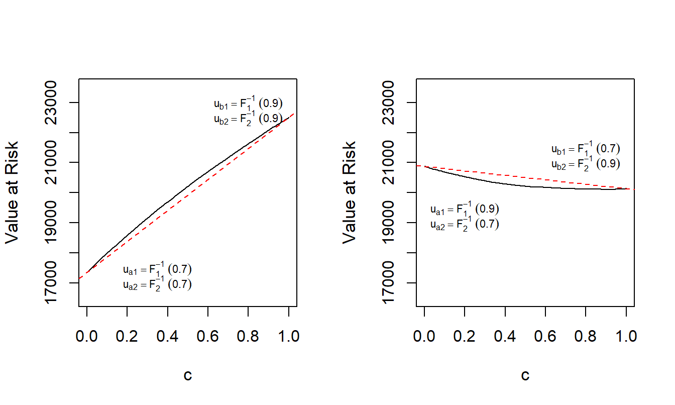
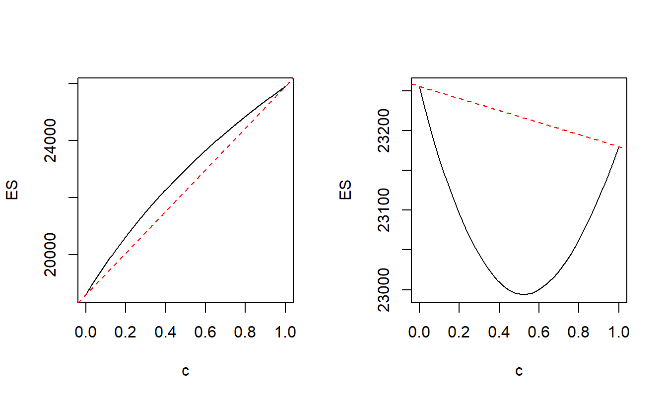
Example 5.1. Lack of Convexity of Value at Risk for Excess of Loss. Suppose that \(X_1\) has a gamma distribution with shape parameter 2 and scale parameter 5,000 so that the mean is 10,000. Suppose that \(X_2\) has a Pareto distribution with shape parameter 5 and scale parameter 25,000 so that the mean is 6,250. The two variables are related through a Gaussian copula with parameter \(\rho=\) -0.3. We seek to evaluate the value at risk with confidence level \(\alpha = 0.90\) for an excess of loss random variable \(S(u_1, u_2) = X_1 \wedge u_1 + X_2 \wedge u_2\), denoted as \(VaR_{0.9}(u_1,u_2)\). We plot \(VaR_{0.9}(u_1,u_2)=VaR_{0.9}({\bf u})\) for various values of \({\bf u} =(u_1,u_2)\).
For the left-hand panel of Figure 5.1, define \({\bf u}_a =(F_1^{-1}(0.7),F_2^{-1}(0.7))\) and \({\bf u}_b =(F_1^{-1}(0.9),F_2^{-1}(0.9))\). Recall the notation that \(F_1^{-1}(0.7)\) denotes the 0.7 quantile of the first distribution (that turns out to be 12,196 for this example). This panel shows a plot of \(VaR_{0.9}[(1-c){\bf u}_a + c {\bf u}_b]\) versus \(c\); the linear interpolation \((1-c)VaR_{0.9}[{\bf u}_a]+ c VaR_{0.9}[{\bf u}_b]\) versus \(c\) is superimposed. Because the graph is above the linear interpolation, the \(VaR\) function is concave over this region.
For the right-hand panel of Figure 5.1, in the same way define \({\bf u}_a =(F_1^{-1}(0.9),F_2^{-1}(0.7))\) and \({\bf u}_b =(F_1^{-1}(0.7),F_2^{-1}(0.9))\). Because the graph is below the linear interpolation, the \(VaR\) function is convex over this region.
In sum, the value at risk function \(VaR_{0.9}({\bf u})\) is neither convex nor concave for all values of \({\bf u} =(u_1,u_2)\) meaning that we cannot use optimization methods that rely on the convexity of a function.
# Example 5.1 Set Up
risk1shape <- 2;           risk1scale <- 5000
risk2shape <- 5         ;  risk2scale <- 25000
rho  <-  -0.3
# Example 5.1 Illustrative Code
nsim <- 200000
set.seed(202020)
#  Normal, or Gaussian, Copula
norm.cop <- copula::normalCopula(param=-0.3, dim = 2,'dispstr' ="un")
UCop     <- copula::rCopula(nsim, norm.cop)
#  Marginal Distributions
X1 <- qgamma(p=UCop[,1],shape = risk1shape, scale = risk1scale)
X2 <- actuar::qpareto(p=(UCop[,2]),shape = risk2shape, scale = risk2scale)
cVec <- seq(0, 1, length.out=200)
u1.0 <- qgamma(p=0.70,shape = risk1shape, scale = risk1scale)
u1.1 <- qgamma(p=0.90,shape = risk1shape, scale = risk1scale)
u2.0 <- actuar::qpareto(p=0.70,shape = risk2shape, scale = risk2scale)
u2.1 <- actuar::qpareto(p=0.90,shape = risk2shape, scale = risk2scale)

u1Vec.a <- u1.0*(1-cVec) + u1.1*cVec
u1Vec.b <- u1.1*(1-cVec) + u1.0*cVec
u2Vec   <- u2.0*(1-cVec) + u2.1*cVec

#  Objective Function
f0 <- function(u1,u2){
      S <- pmin(X1,u1) +  pmin(X2,u2)
      return(quantile(S, probs=0.9))
      }
VarVec.a <- 0* cVec -> VarVec.b
for (kindex in 1:length(cVec)) {
  VarVec.a[kindex] <- f0(u1Vec.a[kindex],u2Vec[kindex])
  VarVec.b[kindex] <- f0(u1Vec.b[kindex],u2Vec[kindex])
}

save(cVec,VarVec.a, VarVec.b,
    file = "../ChapTablesData/Chap5/Example51.Rdata")
# Example 5.1 Illustrative Code, Figure 5.1
# save(cVec,VarVec.a, VarVec.b,
#     file = "../ChapTablesData/Chap5/Example51.Rdata")
load(file = "ChapTablesData/Chap5/Example51.Rdata")

par(mfrow=c(1,2))
  plot(cVec,VarVec.a, type = "l", ylab = "Value at Risk",
     xlab = "c", ylim = c(16500,23500), cex.lab=1.1)
    text(0.35, 17500,  expression(u[a1]==F[1]^-1~(0.7)), cex = 0.7)
    text(0.35, 17000,  expression(u[a2]==F[2]^-1~(0.7)), cex = 0.7)
    text(0.80, 23000,  expression(u[b1]==F[1]^-1~(0.9)), cex = 0.7)
    text(0.80, 22500,  expression(u[b2]==F[2]^-1~(0.9)), cex = 0.7)
    abline(a=VarVec.a[1],b=VarVec.a[length(cVec)]-VarVec.a[1],
       lty = "dashed", col =FigRed)
  plot(cVec,VarVec.b, type = "l", ylab = "Value at Risk",
     xlab = "c", ylim = c(16500,23500), cex.lab=1.1)
    text(0.20, 19500,  expression(u[a1]==F[1]^-1~(0.9)), cex = 0.7)
    text(0.20, 19000,  expression(u[a2]==F[2]^-1~(0.7)), cex = 0.7)
    text(0.80, 21500,  expression(u[b1]==F[1]^-1~(0.7)), cex = 0.7)
    text(0.80, 21000,  expression(u[b2]==F[2]^-1~(0.9)), cex = 0.7)
    abline(a=VarVec.b[1],b=VarVec.b[length(cVec)]-VarVec.b[1],
       lty = "dashed", col =FigRed)
Our interest is in the convexity, or lack thereof, of summary measures of a retained risk. It is important to note that we are thinking of these as functions of risk retention parameters, not as functions of potential losses. That is, it is tempting to think of the realized excess of loss random variable, \(x_1 \wedge u_1 + x_2 \wedge u_2\), as a function of realized losses \(x_1\) and \(x_2\), as is common in applied statistics. In addition, both Examples 5.1 and 5.2 utilize continuous distributions (gamma and Pareto) for losses, mitigating discreteness issues when confirming convexity in the space of potential losses. However, because the interest is in optimization with respect to the risk retention parameter space, we specifically write the excess of loss random variable as \(S(u_1,u_2) =\) \(X_1 \wedge u_1 + X_2 \wedge u_2\) to emphasize our interest in retained loss distributions as a function of risk retention parameters.
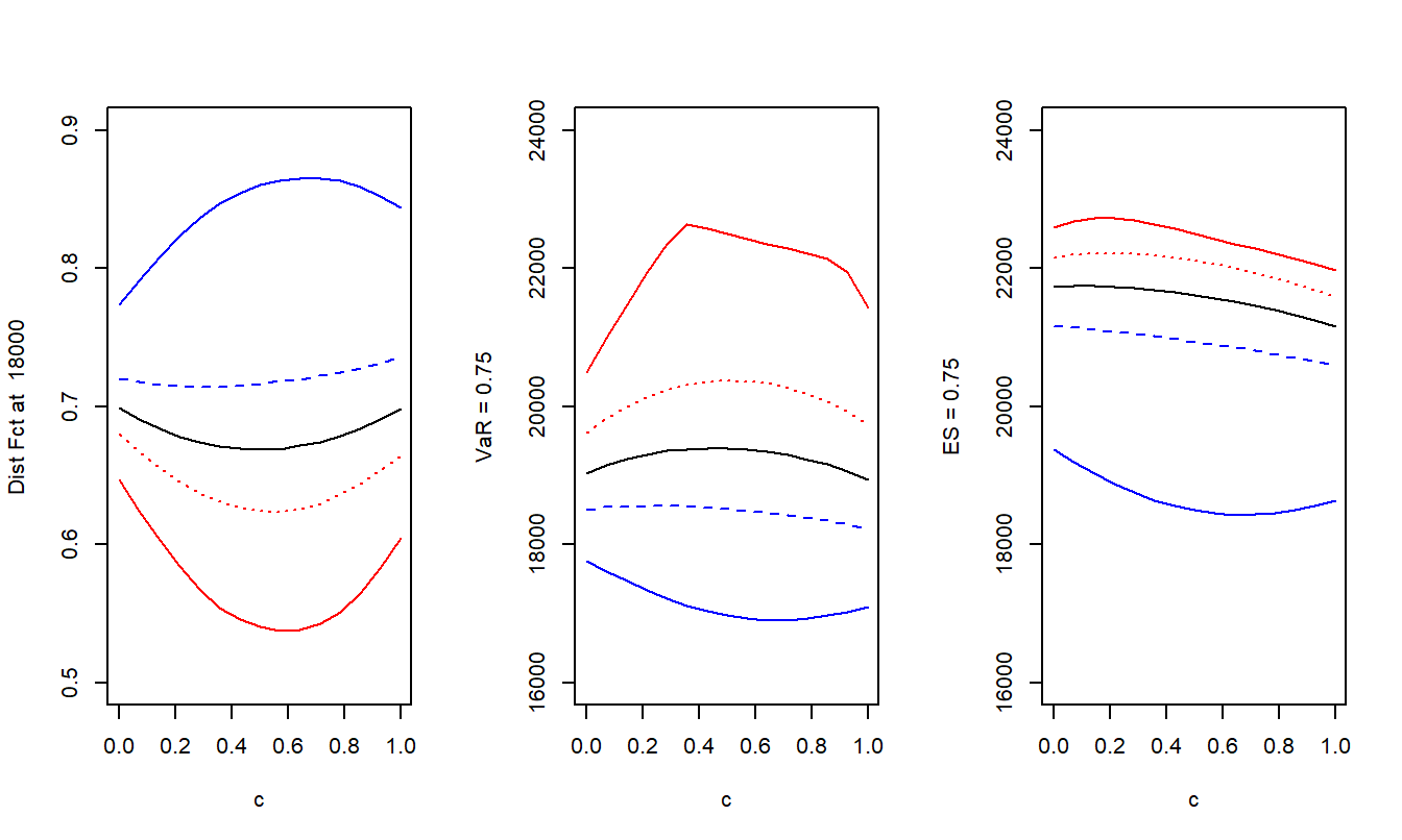
Example 5.2. Three Measures of Uncertainty. This example shows that each of the three measures of uncertainty (the distribution function, quantile, and \(ES\)) is neither convex nor concave for all values of dependence parameters.
To demonstrate this, assume that both \(X_1\) and \(X_2\) have gamma distributions with mean 10,000 and standard deviation 7,071. Their relationship is governed by a normal copula with parameter \(\rho\) that is allowed to vary.
We consider two points, \({\bf u}_a = (8000, 14000)\) and \({\bf u}_b = (16000, 7000)\) and evaluate the distribution function, quantile, and expected shortfall at convex combinations given by \(c {\bf u}_a + (1-c){\bf u}_b\). The distribution function is evaluated at 18,000 and the quantile and expected shortfall use \(\alpha = 0.75\).
Figure 5.2 shows that the convexity depends on the level of dependence. That is, for each measure, sometimes the function is convex and sometimes concave, depending on the dependence. Further, if you do not know about the dependence,
then you do not know whether the function that you are trying to optimize is convex or concave (or neither). As a consequence you may think you are maximizing a function and wind up minimizing it, or vice versa.
# Example 5.2 Set Up
risk1shape <- 2;           risk1scale <- 5000
risk2shape <- 5         ;  risk2scale <- 5000
# Example 5.2 Illustrative Code
nsim <- 200000
# set.seed(2018)
Q          <- 18000
U1Vec      <- c(8000, 14000)
U2Vec      <- c(16000,  7000)
theta      <- seq(from = 0, to = 1, length.out = 15)
uparam     <- matrix(0,nrow=2,ncol=length(theta))
uparam[1,] <- U1Vec[1]*theta + U2Vec[1]*(1-theta)
uparam[2,] <- U1Vec[2]*theta + U2Vec[2]*(1-theta)
#uparam
alpha1     <- 0.75

rhoparam   <- c(-0.9,-.3,0,0.3,0.9)
matrix(0,length(theta),length(rhoparam)) ->
               yQ2 -> QuanS1 -> QuanS2
for (j in 1:length(rhoparam)) {
  set.seed(2018)
  copulaParam <- copula::iRho(normalCopula(param=1, dim = 2),
                              rho=rhoparam[j])
  nc    <- copula::normalCopula(param=copulaParam, dim = 2)
  U     <- copula::rCopula(nsim, nc)
  risk1 <- q1(U[,1])
  risk2 <- q1(U[,2])

  for (i in 1:length(theta)) {
    Retain <- pmin(risk1,uparam[1,i]) + pmin(risk2,uparam[2,i])
    df.2        <- ecdf(Retain)
    yQ2[i,j]    <- df.2(Q)
    quant       <- quantile(Retain, probs = c(alpha1))
    excess      <- pmax(Retain-quant,0)
    CTE         <- quant + mean(excess)/(1-alpha1)
    QuanS1[i,j] <- quant
    QuanS2[i,j] <- CTE
    }
}

save(theta,yQ2,QuanS1,QuanS2,Q,alpha1,
    file = "../ChapTablesData/Chap5/Example52.Rdata")
# Example 5.2 Illustrative Code, Figure 5.2
# save(theta,yQ2,QuanS1,QuanS2,
#     file = "../ChapTablesData/Chap5/Example52.Rdata")
load(file = "ChapTablesData/Chap5/Example52.Rdata")

par(mfrow = c(1,3))
  plot(theta,yQ2[,3], type = "l", ylab=paste("Dist Fct at ",Q),
       ylim=c(0.5,0.9), xlab = "c")
    lines(theta,yQ2[,4],  col=FigRed, lty=3)
        lines(theta,yQ2[,2],  col=FigBlue, lty=2)
lines(theta,yQ2[,5],  col=FigRed, lty=1)
    lines(theta,yQ2[,1],  col=FigBlue, lty=1)

  plot(theta,QuanS1[,3], type = "l", ylab=paste("VaR =",alpha1),
       xlab = "c", ylim = c(16000,24000))
    lines(theta,QuanS1[,4],  col=FigRed, lty=3)
    lines(theta,QuanS1[,2],  col=FigBlue, lty=2)
    lines(theta,QuanS1[,5],  col=FigRed, lty=1)
    lines(theta,QuanS1[,1],  col=FigBlue, lty=1)

  plot(theta,QuanS2[,3], type = "l", ylab=paste("ES =",alpha1),
       xlab = "c", ylim = c(16000,24000))
    lines(theta,QuanS2[,4],  col=FigRed, lty=3)
    lines(theta,QuanS2[,2],  col=FigBlue, lty=2)
    lines(theta,QuanS2[,5],  col=FigRed, lty=1)
    lines(theta,QuanS2[,1],  col=FigBlue, lty=1)
Excess of Loss Distribution
In the bivariate case, there are two risks \(X_1, X_2\). For \(j=1,2\), the distribution of \(X_j\) is \(F_j\) and, when available, the density function is denoted as \(f_j\). The excess of loss retained risk function is \(g(X_1,X_2; \boldsymbol \theta)=\) \(X_1 \wedge u_1 + X_2 \wedge u_2\). For simplicity, this chapter uses the limited sum expression \(S(u_1,u_2) = X_1 \wedge u_1 + X_2 \wedge u_2\) for retained risks.
Distribution Function and Quantiles
Distribution Function. In some detail, I develop the distribution function of \(S(u_1,u_2)\) that can be evaluated at a generic \(y\). First note that if \(y \ge u_1+u_2\), then \(\Pr[S(u_1,u_2) \le y] =1\). So, now consider the case where \(y < u_1+u_2\). On this set, one has
\[\begin{equation}
\begin{array}{ll}
\Pr[S(u_1,&u_2) \le y] \\ ~\\
&= \int_0^{F_1(u_1)} \int_0^{F_2(u_2)} I[F_1^{-1}(z_1) + F_2^{-1}(z_2) \le y]~ c(z_1, z_2) ~ dz_2 dz_1 \\
& \ \ \ + F_2(y-u_1) - C[F_1(u_1),F_2(y-u_1)] \\
& \ \ \ + F_1(y - u_2) - C[F_1(y - u_2),F_2(u_2)] \\ \\
&= \int^{u_1}_{-\infty} C_1[F_1(x), F_2(\min(y-x, u_2))] ~ f_1(x)dx \\
& \ \ \ + F_2(y-u_1) - C[F_1(u_1),F_2(y-u_1)] \\
& \ \ \ + F_1(y - u_2) - C[F_1(y - u_2),F_2(u_2)] .\\
\end{array}
\tag{5.1}
\end{equation}\]
The partial derivative of the copula distribution function, \(C_1(u,v) =\partial_u C(u,v)\), is described in more detail in Appendix Chapter 14. Equation (5.1) is valid for random variables with a domain on the entire real line. Note that if \(X_1\) has a domain on the non-negative portion of the real line and \(u_2>y\), then \(F_1(y-u_2) = 0\), and similarly for \(X_2\). This observation can simplify the calculation.
Going back to the basics, we partition the distribution using the following four sets:
\[
\begin{array}{lcl}
A_1 = \{ X_1 > u_1, X_2 > u_2\}& &
A_2 = \{ X_1 \le u_1, X_2 > u_2\} \\
A_3 = \{ X_1 > u_1, X_2 \le u_2\}& &
A_4 = \{ X_1 \le u_1, X_2 \le u_2\}. \\
\end{array}
\]
At a generic \(y\),or the first set, we have
\[
\begin{array}{ll}
\Pr(S \le y, A_1) &= \Pr(X_1 \wedge u_1 + X_2 \wedge u_2 \le y, X_1 > u_1, X_2 > u_2) \\
&= \Pr(u_1 + u_2 \le y, X_1 > u_1, X_2 > u_2) = I(u_1 + u_2 \le y) \Pr(A_1) \\
&= 0,
\end{array}
\]
because we exclude the case where \(u_1+u_2 \le y\).
For the second set,
\[
\begin{array}{ll}
& \Pr(S \le y, A_2) \\
&= \Pr(X_1 \wedge u_1 + X_2 \wedge u_2 \le y, X_1 \le u_1, X_2 > u_2) \\
&= \Pr(X_1 + u_2 \le y, X_1 \le u_1, X_2 > u_2) =\Pr(X_1 \le y - u_2, X_1 \le u_1, X_2 > u_2)\\
&= \Pr(X_1 \le \min(y-u_2, u_1), X_2 > u_2) = \Pr(X_1 \le y-u_2, X_2 > u_2) \\
&= \Pr(X_1 \le y-u_2) - \Pr(X_1 \le y-u_2, X_2 \le u_2) \\
&= F_1(y-u_2) - C[F_1(y-u_2), F_2(u_2)],
\end{array}
\]
using copula notation. The third line is because \(u_1+u_2 > y\) implies \(\min(y-u_2, u_1) = y-u_2\).
In the same way, for the third set we have
\[
\Pr(S \le y, A_3) = \Pr(X_2 \le y-u_1, X_1 > u_1) =F_2(y-u_1) - C[F_1(u_1),F_2(y-u_1)].
\]
For the fourth set,
\[
\begin{array}{ll}
\Pr(S \le y, A_4) &= \Pr(X_1 \wedge u_1 + X_2 \wedge u_2 \le y, X_1 \le u_1, X_2 \le u_2) \\
&= \Pr(X_1 + X_2 \le y, X_1 \le u_1, X_2 \le u_2) \\
&= \int^{u_1}_{-\infty} \int^{u_2}_{-\infty} I[x_1 + x_2 \le y]f(x_1,x_2)dx_1dx_2 \\
&= \int_0^{F_1(u_1)} \int_0^{F_2(u_2)} I[F_1^{-1}(z_1) + F_2^{-1}(z_2) \le y] c(z_1, z_2) ~ dz_2 dz_1 .
\end{array}
\]
This is sufficient for equation (5.1). For calculation purposes, we also use
\[
\begin{array}{ll}
\Pr(S \le y, A_4) &= \Pr(X_1 + X_2 \le y, X_1 \le u_1, X_2 \le u_2) \\
&= \int^{u_1}_{-\infty} \Pr(X_2 \le y-x, X_2 \le u_2|X_1 = x) f_1(x)dx \\
&= \int^{u_1}_{-\infty} \Pr(X_2 \le \min(y-x, u_2) |X_1 = x) f_1(x)dx \\
&= \int^{u_1}_{-\infty} C_1[F_1(x), F_2(\min(y-x, u_2)] f_1(x)dx ,\\
\end{array}
\]
using the relation
\[
\begin{array}{ll}
\Pr(X_2 \le z |X_1 = x)
&= \frac{\partial_x \Pr(X_2 \le z , X_1 \le x)}{f_1(x)}= \frac{\partial_x C[F_1(x),F_2(z)]}{f_1(x)} \\
&= C_1[F_1(x),F_2(z)] .
\end{array}
\]
See Appendix Chapter 13 for a discussion of derivatives and conditional distributions with copulas.
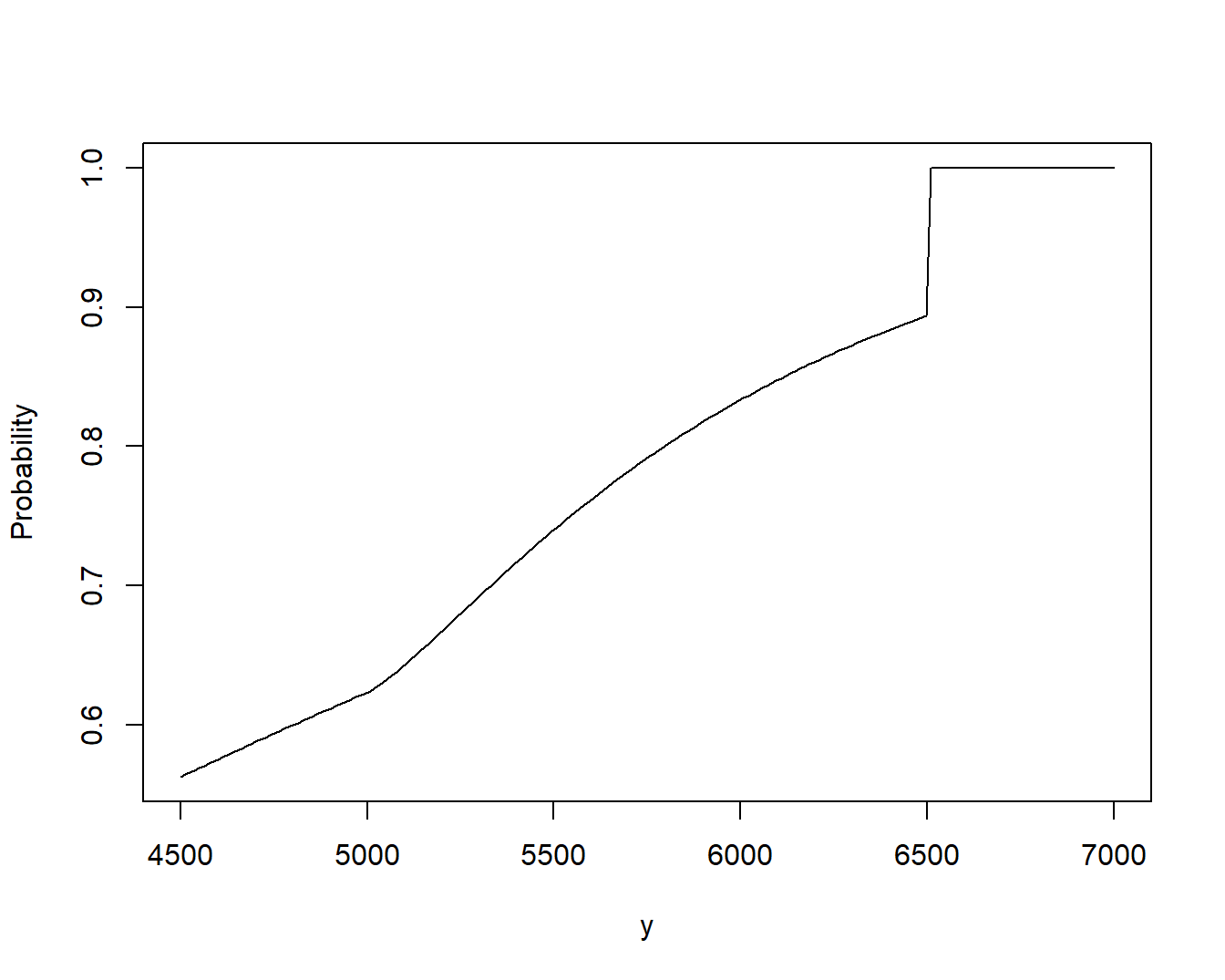
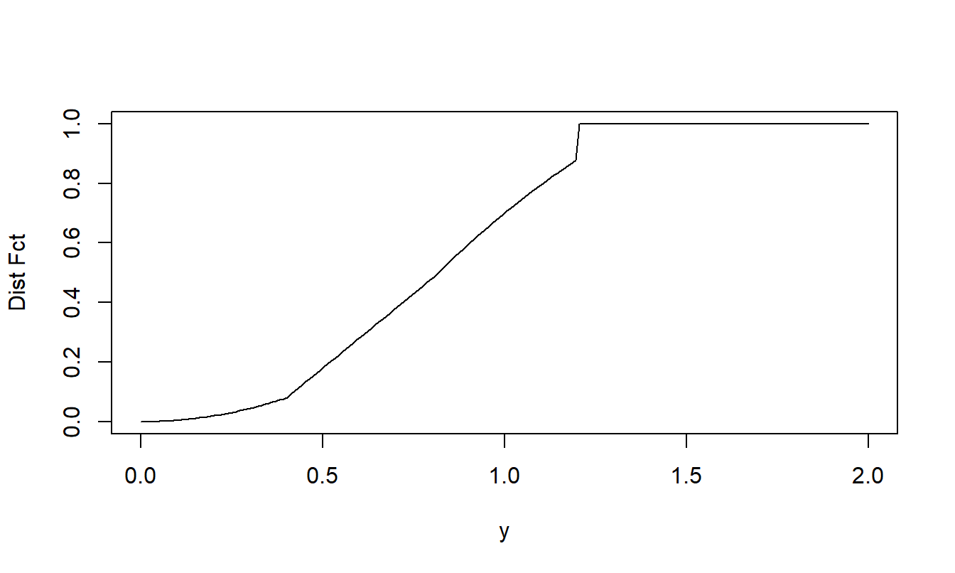
Example 5.3. Bivariate Excess of Loss Distribution. To show the flexibility of this set-up, we use different distributions for the two risks. Specifically, assume that \(X_1\) has a gamma distribution with shape parameter 2 and scale parameter 2,000 and that \(X_2\) has a Pareto distribution with shape parameter 3 and scale parameter 2,000. Their relationship is governed by a normal copula with parameter \(\rho = 0.5\). The code uses \(u_1 = 5,000\) and \(u_2 =1,500\).
Illustrative code shows how to determine the distribution function in two ways, one via integration following the formula in equation (5.1) and one via simulation. Figure 5.3 summarizes the excess of loss distribution function. Even though the two random variables are continuous, note the point of discreteness at \(y=6,500\) where the jump in the distribution function occurs.
# Example 5.3 Set Up
risk1shape <- 2;           risk1scale <- 2000
risk2shape <- 3         ;  risk2scale <- 2000
# These functions are used throughout the book, beginning in Chap 1
# Basic Summary Functions for a gamma Distribution

f1 <- function(x){dgamma(x=x,shape = risk1shape, scale = risk1scale)}
F1 <- function(x){pgamma(q=x,shape = risk1shape, scale = risk1scale)}
q1 <- function(x){qgamma(p=x,shape = risk1shape, scale = risk1scale)}
ERisk1fun  <- function(){actuar::mgamma(order=1, shape = risk1shape,
                                        scale = risk1scale)}
sdRisk1fun <- function(){
       sqrt(actuar::mgamma(order=2, shape = risk1shape,
                           scale = risk1scale) - ERisk1fun()**2)}
RC1 <- function(u){
       ERisk1fun() - actuar::levgamma(limit = u, shape = risk1shape,
                                      scale = risk1scale)}
# Basic Summary Functions for a Pareto Distribution
f2 <- function(x){actuar::dpareto(x=x,shape = risk2shape, scale = risk2scale)}
F2 <- function(x){actuar::ppareto(q=x,shape = risk2shape, scale = risk2scale)}
q2 <- function(x){actuar::qpareto(p=x,shape = risk2shape, scale = risk2scale)}
ERisk2fun  <- function(){actuar::mpareto(order=1, shape = risk2shape,
                                         scale = risk2scale)}
sdRisk2fun <- function(){
      sqrt(actuar::mpareto(order=2, shape = risk2shape,
                           scale = risk2scale) - ERisk2fun()**2)}
RC2 <- function(u){
      ERisk2fun() - actuar::levpareto(limit = u,shape = risk2shape,
                                      scale = risk2scale)}
#  Additive Risk Transfer Cost
RTC <- function(u1,u2){ RC1(u1)+RC2(u2) }
# Chapter 5 Gamma Pareto Functions

Prob.fct <- function(u1,u2,rho,y){
  u1       <- u1*(u1>0)
  u2       <- u2*(u2>0)
  norm.cop <- copula::normalCopula(param=rho, dim = 2,'dispstr' ="un")
  ProbA <- 0 -> ProbB -> ProbC -> ProbD1 -> ProbD2
  if (y>u1) { ProbB <- F2(y-u1) - pCopula(c(F1(u1),F2(y-u1)), norm.cop) }
  if (y>u2) { ProbC <- F1(y-u2) - pCopula(c(F1(y-u2),F2(u2)), norm.cop) }
  ProbD1.x <- function(x){VineCopula::BiCopHfunc1(F1(x),F2(y-x),
                                                  family=1, par=rho)*f1(x)}
  ProbD1.x.vec <- Vectorize(ProbD1.x)
  ProbD1   <-  cubature::cubintegrate(ProbD1.x.vec,
                                      lower = max(0,y-u2), upper = min(y,u1),
                                      relTol =1e-4, absTol =1e-8,
                                      method = "hcubature")$integral
  if (y>u2) { ProbD2 <-  copula::pCopula(c(F1(y-u2),F2(u2)), norm.cop) }
  ProbTot <- ProbA + ProbB + ProbC + ProbD1 + ProbD2
  ProbTot <- ProbTot + (1-ProbTot)*(u1+u2<y)
  ProbTot <- ProbTot*(y>0)
  return(ProbTot)
  }

ExLossESGamPareto <- function(u1,u2,rho,alpha){
    Prob.alpha <- function(y){3e5*(Prob.fct(u1,u2,rho,y) - alpha)}
    VaR        <- uniroot(Prob.alpha, lower = 0, upper = 10e6)$root
    Surv.fct.y <- function(y){1-Prob.fct(u1,u2,rho,y)}
    Surv.fct.y.vec  <- Vectorize(Surv.fct.y)
    Sum.limited.Var <- integrate(Surv.fct.y.vec, lower = 0,
                                 upper = VaR)$value
    TotalRetained   <- actuar::levgamma(limit = u1,shape = risk1shape,
                                        scale = risk1scale) +
                       actuar::levpareto(limit = u2,shape = risk2shape,
                                         scale = risk2scale)
    ES        <- VaR + (TotalRetained- Sum.limited.Var)/(1-alpha)
    Output     <- list(Prob.fct(u1,u2,rho, y=4.5*RTCmax), VaR, ES)
    return(Output)
    }
# Example 5.3 Illustrative Code, Figure 5.3
#  No Constraints

#  Determine the Probability
u1<-5000;u2 <- 1500; rho<-0.5;
Probsumarg <- seq(max(u1,u2)-500, u1+u2+500, length.out=200)
Probsum    <- 0*Probsumarg
for (kindex in 1:length(Probsumarg)) {
    Probsum[kindex] <- Prob.fct(u1,u2,rho, Probsumarg[kindex]) }
plot(Probsumarg,Probsum, type="l", ylab="Probability", xlab="y" )
# Example 5.3 Illustrative Code
# Check Using Simulation
nsim      <- 1000000
rGaus     <- matrix(rnorm(2*nsim),nrow=nsim,ncol=2)
rho       <- 0.5
Sigma.11  <- matrix(c(1,rho,rho,1),nrow=2,ncol=2)
rGaus.new <- rGaus %*% chol(Sigma.11)
UCop1     <- pnorm(rGaus.new[,1])
UCop2     <- pnorm(rGaus.new[,2])
#  Marginal Distribution Random variables
X1 <- qgamma(p=UCop1,shape = risk1shape, scale = risk1scale)
X2 <- actuar::qpareto(p=UCop2,shape = risk2shape,
                      scale = risk2scale)
S <- pmin(X1,u1) +  pmin(X2,u2)
# Checks out well
# mean((S <= 6000))
# Prob.fct(u1,u2,rho, 6000)
Quantiles. The R code shows how to determine quantiles (value at risk) for the excess of loss distribution in three ways:
- using the formula in equation (5.1) with the
R uniroot function,
- via simulation, and
- as a constrained optimization approach that will be presented in Section 7.2.
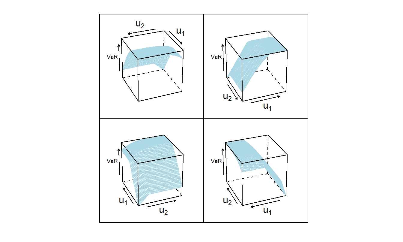
I use the distribution and parameter values from Example 5.3 and \(\alpha = 0.85\). It turns out that the quantile is approximately 6,116. Figure 5.4 summarizes the quantile as a function of the two upper limits with a three-dimensional figure, shown from several perspectives.
# Example 5.3 Illustrative Code
#  Determine the Quantile
u1 <- 5000; u2 <- 1500; rho <- 0.5; alpha <- 0.85;
Prob.alpha <- function(Quan){Prob.fct(u1,u2,rho,Quan) - alpha}
QuanAlpha  <- uniroot(Prob.alpha, lower = 0, upper = 10e6)$root
# Simulation
#QuanAlphasim <- quantile(S, probs = alpha, na.rm = TRUE)
# Constrained Optimization Approach
y.Vec <- function(par){par[1]}
Prob.y.Vec <- function(par){
  y=par[1]
  return(1e6*(Prob.fct(u1,u2,rho,y) - alpha))
  }
f0Prob.opt <-
  auglag(par=7000,                   # initial value
         fn=y.Vec,                   # objective function
         hin=Prob.y.Vec,             # inequality constraint
         control.outer=list(method="nlminb",trace=FALSE, itmax=20),
         control.optim=list(maxit=20))
#QuanAlpha;QuanAlphasim;f0Prob.opt$value
# Nice
# Example 5.3 Set Up
risk1shape <- 2;           risk1scale <- 2000
risk2shape <- 3         ;  risk2scale <- 2000
# Example 5.3 Illustrative Code
# This code generates the VaR and ES over a grid of values of u1 and u2
# Done for corr = 0.5 and corr = -0.5
# Results are stored in and .RData file for later use....
TimeNeg   <- Sys.time()

alpha  <-  0.85
rho    <- 0.50

gridsize <- 50
u1Vec <-
  seq(qgamma(p=0.01,shape = risk1shape, scale = risk1scale),
      qgamma(p=0.99,shape = risk1shape, scale = risk1scale),
      length.out=gridsize)
u2Vec <-
  seq(actuar::qpareto(p=0.01,shape = risk2shape, scale = risk2scale),
      actuar::qpareto(p=0.99,shape = risk2shape, scale = risk2scale),
      length.out=gridsize)

RMGridPos <- matrix(0,gridsize**2,5)
count = 0
for (i in 1:gridsize)
  {for (j in 1:gridsize) {
    count = count + 1
  RMGridPos[count,1] <- u1Vec[i]
  RMGridPos[count,2] <- u2Vec[j]
  T1 <- ExLossESGamPareto(u1=u1Vec[i],u2=u2Vec[j],rho,alpha)
  RMGridPos[count,3] <- T1[[2]]
  RMGridPos[count,4] <- T1[[3]]
  RMGridPos[count,5] <- RC1(u1Vec[i]) + RC2(u2Vec[j])
  }}
colnames(RMGridPos) <- c("u1", "u2", "VaR", "ES", "RTC")
RMGridPos <- data.frame(RMGridPos)
save(RMGridPos,
     file = "../ChapTablesData/Chap5/Example521PosCorr.RData")

#Rerun with negative correlation
TimeNeg   <- Sys.time()
rho       <- -0.5;
RMGridNeg <- matrix(0,gridsize**2,5)
count     <-  0
for (i in 1:gridsize)
  {for (j in 1:gridsize) {
    count  <-  count + 1
  RMGridNeg[count,1] <- u1Vec[i]
  RMGridNeg[count,2] <- u2Vec[j]
  T1 <- ExLossESGamPareto(u1=u1Vec[i],u2=u2Vec[j],rho,alpha)
  RMGridNeg[count,3] <- T1[[2]]
  RMGridNeg[count,4] <- T1[[3]]
  RMGridNeg[count,5] <- RC1(u1Vec[i]) + RC2(u2Vec[j])
  }}

colnames(RMGridNeg) <- c("u1", "u2", "VaR", "ES", "RTC")
RMGridNeg <- data.frame(RMGridNeg)
save(RMGridNeg,
     file = "../ChapTablesData/Chap5/Example521NegCorr.RData")
Sys.time() - TimeNeg
#Time difference of 3.11391334 hours
# Example 5.3 Illustrative Code, Figure 5.4
# save(RMGridPos,
#      file = "../ChapTablesData/Chap5/Example521PosCorr.RData")
load( file = "ChapTablesData/Chap5/Example521PosCorr.RData")

angle <- 22+c(0, 90, 180,270)
#angle <- c( 160, 240, 110, 20)
Angle <- shingle(rep(angle, rep(length(RMGridPos[,3]), 4)),angle)

wireframe(rep(RMGridPos[,3], 4) ~
          rep(RMGridPos[,2], 4) *rep(RMGridPos[,1], 4) | Angle,
          groups = Angle,
  panel = function(x, y, subscripts, z, groups,...){
    w <- groups[subscripts][1]
    panel.wireframe(x, y, subscripts, z,
    screen = list(z = w, x = -60, y = 0), ...)},
  strip = FALSE,
  par.settings = list(par.zlab.text=list(cex = 0.6)),
  skip = c(F, F, F, F),
  layout = c(2,2),#shade=TRUE,
  distance = 0.1, col = FigLBlue,
  xlab = expression(u[2]), ylab = expression(u[1]),
  zlab = "VaR")
Partial Derivatives of Distribution Functions
Partial Derivatives of the Distribution Function. I next develop partial derivatives of the distribution function. Based on equation (5.1), one can establish
\[\begin{equation}
\begin{array}{ll}
\partial_{u_1} &\Pr[S(u_1,u_2) \le y] \\
& = - f_2(y-u_1)\left\{1-C_2[F_1(u_1),F_2(y-u_1)] \right\} .\\
\end{array}
\tag{5.2}
\end{equation}\]
Taking a partial derivative of the first line of equation (5.1), we have
\[
\begin{array}{ll}
\frac{\partial}{\partial u_1} & \int_0^{F_1(u_1)} \int_0^{F_2(u_2)} I[F_1^{-1}(z_1) + F_2^{-1}(z_2) \le y] c(z_1, z_2) ~ dz_2 dz_1 \\
& = f_1(u_1)\int_0^{F_2(u_2)} I[u_1 + F_2^{-1}(z_2) \le y] ~c[F_1(u_1), z_2] ~ dz_2 \\
& = f_1(u_1)\int_0^{F_2(u_2)\wedge F_2(y-u_1)} c[F_1(u_1), z_2] ~ dz_2 \\
& = f_1(u_1) ~C_1[F_1(u_1), F_2(y-u_1)] ,\\
\end{array}
\]
with \(y-u_1 < u_2\).
Taking a partial derivative of the second line of equation (5.1) yields
\[
\begin{array}{ll}
\partial_{u_1}& \left\{F_2(y-u_1) - C[F_1(u_1),F_2(y-u_1)] \right\} \\
& = -f_2(y - u_1) - \partial_{u_1} \left\{C[F_1(u_1),F_2(y-u_1)]\right\} \\
& = -f_2(y - u_1) \\
& \ \ \ \ - \left\{f_1(u_1)C_1[F_1(u_1),F_2(y-u_1)]-f_2(y-u_1)C_2[F_1(u_1),F_2(y-u_1)]\right\} \\
& = - f_1(u_1) C_1[F_1(u_1), F_2(y-u_1)]-f_2(y-u_1)\left\{1-C_2[F_1(u_1),F_2(y-u_1)] \right\} .\\
\end{array}
\]
Adding these two results is sufficient for equation (5.2).
Note that this partial derivative is 0 for \(u_1>y\) and non-negative \(X_2\). Intuitively, for large upper limits \(u_1\), changes in \(u_1\) do not affect the distribution function. Now, in the same way,
\[\begin{equation}
\begin{array}{ll}
\partial_{u_2} & \Pr[S(u_1,u_2) \le y] \\
& = - f_1(y-u_2) \left\{1-C_2[F_2(u_2),F_1(y-u_2)] \right\} .\\
\end{array}
\tag{5.3}
\end{equation}\]
This presentation assumes a copula symmetric in its arguments so that \(C(u_1,u_2)=C(u_2,u_1)\). For symmetric copulas, one has
\[
C_1(u_1,u_2)=\partial_{u_1}C(u_1,u_2)=\partial_{u_1}C(u_2,u_1)=C_2(u_2,u_1).
\]
This assumption serves to ease some of the computational aspects, as follows.
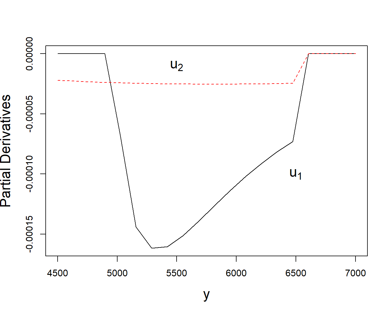
Example 5.4. Partial Derivatives of Bivariate Excess of Loss Distribution Function. This is a continuation of Example 5.3. To illustrate, a block of code is available that shows how to evaluate the partial derivatives. The resulting values are corroborated using numerical approximations from the R function grad. Using the distribution and parameter values from Example 5.3 and \(\alpha = 0.85\), Figure 5.5 summarizes the behavior of these partial derivatives.
# Example 5.4 Illustrative Code
#  No Constraints
PDeriv.fct <- function(u1,u2,rho,y){
  u1        <- u1*(u1>0)
  u2        <- u2*(u2>0)
  norm.cop  <- copula::normalCopula(param=rho, dim = 2,'dispstr' ="un")
  PDeriv.u1 <- -((u1<y)*f2(y-u1)*(1 -
    VineCopula::BiCopHfunc2(F1(u1),F2(y-u1), family=1, par=rho)) )*(u1+u2>y)
  PDeriv.u2 <- -((u2<y)*f1(y-u2)*(1 -
    VineCopula::BiCopHfunc2(F2(u2),F1(y-u2), family=1, par=rho)) )*(u1+u2>y)
  return(c(PDeriv.u1,PDeriv.u2))
  }

#  Plot the Partial Derivatives
u1 <- 5000;u2 <- 1500; rho <- 0.5;
PDeriv.arg <- seq(max(u1,u2)-500, u1+u2+500, length.out=20)
PDeriv.u1  <- 0*PDeriv.arg -> PDeriv.u2
for (kindex in 1:length(PDeriv.arg)) {
  PDeriv.u1[kindex] <- PDeriv.fct(u1,u2,rho, PDeriv.arg[kindex])[1]
  PDeriv.u2[kindex] <- PDeriv.fct(u1,u2,rho, PDeriv.arg[kindex])[2]
  }
plot(PDeriv.arg,PDeriv.u1, type="l",
     ylab="Partial Derivatives", xlab="y", cex.lab=1.5 )
  lines(PDeriv.arg, PDeriv.u2, col = FigRed , lty =2)
  text(6500,-0.00010, expression(u[1]), cex=1.5)
  text(5500,-0.00001, expression(u[2]), cex=1.5)

#  Determine the Partial Derivative Using Numerical Approximation
Prob.fct.Vec <- function(par,rho){Prob.fct(par[1],par[2],par[3],par[4])}
#  Agreement in these two approaches
#numDeriv::grad(f=Prob.fct.Test.Vec, x = c(5000,1500))
# numDeriv::grad(f=Prob.fct.Vec, x = c(5000,1500,0.5,6000))
# PDeriv.fct(5000,1500,0.5,6000)
Second-Order Partial Derivatives of the Distribution Function. Note that the partial derivatives in equations (5.2) and (5.3) are functions of a single upper limit, so the derivative with respect to both parameters is zero. One can also determine
\[\begin{equation}
{\small
\begin{array}{lll}
& \partial^2_{u_1} \Pr[S(u_1,u_2) \le y] \\
& = -\partial_{u_1} \left[f_2(y-u_1)\left\{1-C_2[F_1(u_1),F_2(y-u_1)] \right\} \right]\\
& = \left[f_2^{\prime}(y-u_1)\left\{1-C_2[F_1(u_1),F_2(y-u_1)] \right\} \right.\\
& \ \ \ \ \ \ \ \ \ \ \ \ \ \ \ \ \ \ + f_2(y-u_1)\{c[F_1(u_1),F_2(y-u_1)]f_1(u_1) \\
& \ \ \ \ \ \ \ \ \ \ \ \ \ \ \ \ \ \ \ \ \ \ \ \ \ \ \ \ \ \ \ \ \ \ \ \ \ \ \left. -C_{22}[F_1(u_1),F_2(y-u_1)]f_2(y-u_1)\} \right] .\\
\end{array}
}
\tag{5.4}
\end{equation}\]
Switch the indices to get an expression for \(\frac{\partial^2}{\partial u_2^2} \Pr[S(u_1,u_2) \le y]\).
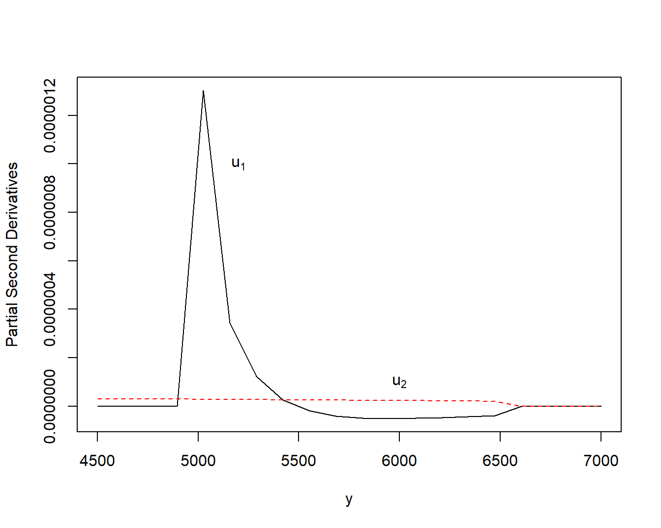
Example 5.5. Second Partial Derivatives of Bivariate Excess of Loss Distribution Function. This is a continuation of Example 5.4. To illustrate, a block of code is available that shows how to evaluate the partial second derivatives. The resulting values are corroborated using numerical approximations from the R functions grad and hessian. Using the distribution and parameter values from Example 5.3 and \(\alpha = 0.85\), Figure 5.6 shows the behavior of these partial second derivatives.
# Example 5.5 Illustrative Code
f2prime <- function(y){-f2(y)*(risk2shape+1)/(y+risk2scale) }
f1prime <- function(y){
           ( (risk1shape-1)/y - 1/risk1scale )*f1(y)
           }
C22    <- function(v1,v2,rho){
          z1  <- qnorm(v1)
          z2  <- qnorm(v2)
          arg <- (z1 - rho*z2)/sqrt(1 - rho*rho)
          C22.v1v2 <- - rho/(sqrt(1 - rho*rho)*dnorm(z2))*dnorm(arg)
          return(C22.v1v2)
          }
PSecDeriv.fct <- function(u1,u2,rho,y){
    u1       <- u1*(u1>0)
    u2       <- u2*(u2>0)
    norm.cop <- copula::normalCopula(param=rho, dim = 2,'dispstr' ="un")
    PSecDeriv.u1 <- f2prime(y-u1)*(1 -
       VineCopula::BiCopHfunc2(F1(u1),F2(y-u1), family=1, par=rho) ) +
       f2(y-u1)*dCopula(c(F1(u1),F2(y-u1)), norm.cop)*f1(u1) -
       f2(y-u1)*C22(F1(u1),F2(y-u1),rho)*f2(y-u1)
    PSecDeriv.u1 <- PSecDeriv.u1*(u1+u2>y)
    if (y<u1) PSecDeriv.u1 <- 0
    PSecDeriv.u2 <- f1prime(y-u2)*(1 -
          VineCopula::BiCopHfunc2(F2(u2),F1(y-u2), family=1, par=rho)) +
       f1(y-u2)*dCopula(c(F2(u2),F1(y-u2)), norm.cop)*f2(u2) -
       f1(y-u2)*C22(F2(u2),F1(y-u2),rho)*f1(y-u2)
    PSecDeriv.u2 <- PSecDeriv.u2*(u1+u2>y)
    if (y<u2) PSecDeriv.u2 <- 0
    return(c(PSecDeriv.u1,PSecDeriv.u2))
  }

#  Plot the Partial Derivatives
#u1=5000;u2 = 1500; y=4000;rho=0.5; PSecDeriv.fct(u1,u2, y)
PSecDeriv.arg <- seq(max(u1,u2)-500, u1+u2+500, length.out=20)
PSecDeriv.u1 <- 0*PSecDeriv.arg -> PSecDeriv.u2
for (kindex in 1:length(PSecDeriv.arg)) {
PSecDeriv.u1[kindex] <-
  PSecDeriv.fct(u1,u2,rho, PSecDeriv.arg[kindex])[1]
PSecDeriv.u2[kindex] <-
  PSecDeriv.fct(u1,u2,rho, PSecDeriv.arg[kindex])[2]
}
plot(PSecDeriv.arg,PSecDeriv.u1, type="l",
     ylab="Partial Second Derivatives", xlab="y" )
lines(PSecDeriv.arg, PSecDeriv.u2, col = FigRed , lty =2)
text(5200, 0.0000010, expression(u[1]))
text(6000, 0.0000001, expression(u[2]))

#  Determine the Partial Second Derivatives Using Numerical Approximations
#  Agreement in these two approaches
# testpoint <- c(5000,1500,0.5,6000)
# PDeriv.fct.Vec.u1 <- function(par){PDeriv.fct(par[1],par[2],0.5,6000)[1]}
# PDeriv.fct.Vec.u2 <- function(par){PDeriv.fct(par[1],par[2],0.5,6000)[2]}
# 1e7*numDeriv::hessian(f=Prob.fct.Test.Vec, x = c(5000,1500))
# 1e7*numDeriv::hessian(f=Prob.fct.Vec, x = testpoint )
#  #  Note that cross-partial derivatives are incorrect numerically.
#  #  This is due to the boundary induced by u1 + u2 > y. Safe to ignore.
# 1e7*numDeriv::grad(f=PDeriv.fct.Vec.u1, x = testpoint)[1]
# 1e7*numDeriv::grad(f=PDeriv.fct.Vec.u2, x = testpoint)[2]
# 1e7*PSecDeriv.fct(5000,1500,0.5,6000)

# To check using simulation, need to increase the number of simulations,
# testpointA <- c(5000,1500,6000)
# Prob.Sim.Vec <- function(par){
#    S <- pmin(X1,par[1]) +  pmin(X2,par[2])
#    mean((S <= par[3]))}
# Prob.Sim.Vec(testpointA)
# Prob.fct.Vec(testpoint)
# 1e7*numDeriv::jacobian(f=Prob.Sim.Vec, x = testpointA)
# 1e7*numDeriv::jacobian(f=Prob.fct.Vec, x = testpoint)
# 1e7*numDeriv::hessian(f=Prob.Sim.Vec, x = testpointA)
# 1e7*numDeriv::hessian(f=Prob.fct.Vec, x = testpoint)
Risk Measure Sensitivities
As described in Section 2.1, the uncertainty of retained risks can be summarized using a risk measure. Further, Section 2.3.2 showed how to compute
\[
\partial_{\theta} ~VaR_{\alpha}[g(X; \theta)] ~~~\text{and}~~~\partial_{\theta} ~ES_{\alpha}[g(X; \theta)],
\]
that is, the differential change in these risk measures per unit change in the parameter \(\theta\). The motivation is that it seems reasonable to want to know how such summary measures change in response to (small) changes in the risk retention parameters. The problems in Section 2.3.2 were rather specialized, with only a single random variable \(X\) and parameter \(\theta\). By making some mild additional assumptions to ensure smoothness, we are able to handle many additional situations. let us first introduce a general framework, and then specialize it to the two-risk excess of loss case.
Quantile Sensitivities
Specifically, now consider a generic random vector \(\mathbf{X}\) and let \(g(\mathbf{X}; \boldsymbol \theta)\) be a retention function that depends on outcomes in \(\mathbf{X}\) and a vector of parameters \(\boldsymbol \theta\). Let \(\Pr[ g(\mathbf{X};\boldsymbol \theta) \le y] = F(\boldsymbol \theta; y)\) be the distribution function of the random variable \(g(\mathbf{X};\boldsymbol \theta)\) with corresponding density function \(f(\boldsymbol\theta; \cdot)\). For fixed \(\boldsymbol \theta\), denote the inverse function at \(\alpha\) to be \(VaR_{\alpha}(\boldsymbol \theta)=VaR(\boldsymbol \theta)\), the value at risk (suppressing the explicit dependence on \(\alpha\)).
Assume sufficient local smoothness of \(F(\boldsymbol \theta; y)\) in both arguments \(y\) and \(\boldsymbol \theta\) to permit taking partial derivatives with respect to these arguments. Then, one can use calculus to develop the quantile sensitivity,
\[\begin{equation}
\begin{array}{ll}
\partial_{\boldsymbol \theta}VaR(\boldsymbol \theta) &=
\frac{-1}{F_y[\boldsymbol \theta; VaR(\boldsymbol \theta)]} F_{\boldsymbol \theta}[\boldsymbol \theta; VaR(\boldsymbol \theta)] .
\end{array}
\tag{5.5}
\end{equation}\]
Here, I use \(F_{\boldsymbol \theta}[\boldsymbol \theta; y] = \partial_{\boldsymbol \theta}F[\boldsymbol \theta; y]\) for the vector of partial derivatives with respect to \(\boldsymbol \theta\) and similarly for \(F_y\). Further, the matrix of second derivatives of the value at risk turns out to be
\[\begin{equation}
{\small
\begin{array}{ll}
&\partial_{\boldsymbol \theta} \partial_{\boldsymbol \theta^{\prime}} VaR(\boldsymbol \theta) \\
&= \frac{-1}{F_{y}[\boldsymbol \theta; VaR(\boldsymbol \theta)]}
\left\{F_{\boldsymbol \theta\boldsymbol \theta^{\prime}}[\boldsymbol \theta; VaR(\boldsymbol \theta)]+
F_{y y}[\boldsymbol \theta; VaR(\boldsymbol \theta)] \times
\partial_{\boldsymbol \theta}VaR(\boldsymbol \theta)
\partial_{\boldsymbol \theta^{\prime}}VaR(\boldsymbol \theta)
\right. \\
& ~~~~~~~
+ \left. \partial_{\boldsymbol \theta}VaR(\boldsymbol \theta) \times F_{y \boldsymbol \theta^{\prime}}[\boldsymbol \theta; VaR(\boldsymbol \theta)]
+ F_{y \boldsymbol \theta}[\boldsymbol \theta; VaR(\boldsymbol \theta)] \times \partial_{\boldsymbol \theta^{\prime}}VaR(\boldsymbol \theta) \right\} .\\
\end{array}
}
\tag{5.6}
\end{equation}\]
We assume local smoothness of \(F(\boldsymbol \theta,y)\) in both arguments \(y\) and \(\theta\) so that \(constant = F[\boldsymbol \theta,VaR(\boldsymbol \theta)]\) locally. Differentiating with respect to \(\boldsymbol \theta\) yields
\[
\begin{array}{ll}
0 &= \partial_{\boldsymbol \theta} F[\boldsymbol \theta,VaR(\boldsymbol \theta)] \\
& = \left. \partial_{\boldsymbol \theta} F[\boldsymbol \theta,y]\right|_{y=VaR(\boldsymbol \theta)}
+ \left. \partial_{y} F[\boldsymbol \theta,y]\right|_{y=VaR(\boldsymbol \theta)} \times \partial_{\boldsymbol \theta}VaR(\boldsymbol \theta)\\
& = \left. F_{\boldsymbol \theta}[\boldsymbol \theta,y]\right|_{y=VaR(\boldsymbol \theta)}
+ \left. F_y[\boldsymbol \theta,y]\right|_{y=VaR(\boldsymbol \theta)} \times \partial_{\boldsymbol \theta}VaR(\boldsymbol \theta)\\
& = F_{\boldsymbol \theta}[\boldsymbol \theta,VaR(\boldsymbol \theta)]
+ F_y[\boldsymbol \theta,VaR(\boldsymbol \theta)] \times \partial_{\boldsymbol \theta}VaR(\boldsymbol \theta).
\end{array}
\]
This is sufficient for equation (5.5).
Taking partial derivatives again, for the first term, we have
\[
\begin{array}{ll}
& \partial_{\boldsymbol \theta} F_{\boldsymbol \theta^{\prime}}[\boldsymbol \theta,VaR(\boldsymbol \theta)] = F_{\boldsymbol \theta\boldsymbol \theta^{\prime}}[\boldsymbol \theta,VaR(\boldsymbol \theta)]
+ \partial_{\boldsymbol \theta}VaR(\boldsymbol \theta) \times F_{y\boldsymbol \theta^{\prime} }[\boldsymbol \theta,VaR(\boldsymbol \theta)] .
\end{array}
\]
For the second term, we have
\[
\begin{array}{ll}
& \partial_{\boldsymbol \theta}
\left\{F_y[\boldsymbol \theta,VaR(\boldsymbol \theta)] \times \partial_{\boldsymbol \theta^{\prime}}VaR(\boldsymbol \theta)
\right\} \\
&= \left\{\partial_{\boldsymbol \theta} ~F_y[\boldsymbol \theta,VaR(\boldsymbol \theta)] \right\}
\times
\partial_{\boldsymbol \theta^{\prime}}VaR(\boldsymbol \theta)
+ F_y[\boldsymbol \theta,VaR(\boldsymbol \theta)] \times \partial_{\boldsymbol \theta}\partial_{\boldsymbol \theta^{\prime}}VaR(\boldsymbol \theta) \\
&=\left\{
F_{\boldsymbol \theta y}[\boldsymbol \theta,VaR(\boldsymbol \theta)] +
F_{y y}[\boldsymbol \theta,VaR(\boldsymbol \theta)] \partial_{\boldsymbol \theta}VaR(\boldsymbol \theta)
\right\} \times \partial_{\boldsymbol \theta^{\prime}}VaR(\boldsymbol \theta) \\
& \ \ \ \ + F_{y}[\boldsymbol \theta, VaR(\boldsymbol \theta)] \times \partial_{\boldsymbol \theta} \partial_{\boldsymbol \theta^{\prime}}VaR(\boldsymbol \theta) .
\end{array}
\]
Putting this together, the matrix of second derivatives of the quantile, or value at risk, is as in equation (5.6).
Special Case. Two Risk Excess of Loss. In this case, the vector of parameters is \(\boldsymbol \theta = (u_1,u_2)^{\prime}\) and the retained risk function is the limited sum \(S(u_1,u_2)= X_1 \wedge u_1 + X_2 \wedge u_2\). The distribution function, density, density derivative, and quantile are:
\[
\begin{array}{ll}
F(\boldsymbol \theta; y) &= F(u_1, u_2;y) = \Pr[S(u_1,u_2) \le y] \\
F_y(\boldsymbol \theta; y) &= \partial_y ~ F(\boldsymbol \theta; y) = \partial_y ~ F(u_1, u_2;y) \\
F_{yy}(\boldsymbol \theta; y) &= \partial_y^2 ~ F(\boldsymbol \theta; y) = \partial_y^2 ~ F(u_1, u_2;y) \\
VaR(\boldsymbol \theta) &=F^{-1}_{\alpha}(u_1, u_2).
\end{array}
\]
From equations (5.2) and (5.3), the vector of first derivatives with respect to parameters of the distribution function is
\[
\begin{array}{ll}
F_{\boldsymbol \theta}(\boldsymbol \theta; y) & =F_{u_1, u_2}(u_1, u_2;y) \\
& =
\left(
\begin{array}{c}
- f_2(y-u_1)\left\{1-C_2[F_1(u_1),F_2(y-u_1)] \right\}\\
- f_1(y-u_2) \left\{1-C_2[F_2(u_2),F_1(y-u_2)] \right\}
\end{array}
\right) .
\end{array}
\]
Taking another partial derivative, one has
\[
\begin{array}{ll}
F_{\boldsymbol \theta y}(\boldsymbol \theta; y) & = \partial_y F_{u_1, u_2}(u_1, u_2; y) \\
&=
\left(
\begin{array}{c}
- \left[ f_2^{\prime}(y-u_1)\left\{1-C_2[F_1(u_1),F_2(y-u_1)] \right\} \right.\\
\left. - f_2^2(y-u_1)C_{22}[F_1(u_1),F_2(y-u_1)] \right]\\
- \left[ f_1^{\prime}(y-u_2) \left\{1-C_2[F_2(u_2),F_1(y-u_2)] \right\} \right.\\
-\left. f_1^2(y-u_2) C_{22}[F_2(u_2),F_1(y-u_2)] \right]\\
\end{array}
\right) .
\end{array}
\]
The matrix of second derivatives with respect to parameters of the distribution function is
\[
F_{\boldsymbol \theta\boldsymbol \theta^{\prime}}(\boldsymbol \theta; y) =
\left(
\begin{array}{cc}
\partial^2_{u_1} F(u_1,u_2;y) & 0 \\
0 & \partial^2_{u_2} F(u_1,u_2;y)\\
\end{array}
\right) ,
\]
where the diagonal elements are given in equation (5.4).
# Section 5.3.1 Illustrative Code, on Quantile Derivatives...
# f2prime <- function(y){ -f2(y)*(risk2shape+1)/(y+risk2scale) }
f1prime <- function(y){ ((risk1shape-1)/y - 1/risk1scale)*f1(y) }

CrossPDeriv.fct <- function(u1,u2,rho,y){
  u1       <- u1*(u1>0)
  u2       <- u2*(u2>0)
  norm.cop <- copula::normalCopula(param=rho, dim = 2,'dispstr' ="un")
  PSecDeriv.u1.y <-
    f2prime(y-u1)*(1 -
      VineCopula::BiCopHfunc2(F1(u1),F2(y-u1), family=1, par=rho)) +
    - f2(y-u1)**2*C22(F1(u1),F2(y-u1),rho)
  PSecDeriv.u1.y <- -PSecDeriv.u1.y*(u1+u2>y)
  if (y<u1) PSecDeriv.u1.y <- 0
  PSecDeriv.u2.y <-
    f1prime(y-u2)*(1 -
      VineCopula::BiCopHfunc2(F2(u2),F1(y-u2), family=1, par=rho)) +
    f1(y-u2)*dCopula(c(F2(u2),F1(y-u2)), norm.cop)*f2(u2) -
    f1(y-u2)**2*C22(F2(u2),F1(y-u2),rho)
  PSecDeriv.u2.y <- -PSecDeriv.u2.y*(u1+u2>y)
  if (y<u2) PSecDeriv.u2.y <- 0
  return(c(PSecDeriv.u1.y,PSecDeriv.u2.y))
  }

ExLossCTE <- function(u1,u2,rho,alpha){
# See Section 5.6 for Theory underpinning ES derivatives
    Prob.alpha    <- function(y){Prob.fct(u1,u2,rho,y) - alpha}
    VaR           <- uniroot(Prob.alpha, lower = 0, upper = 10e6)$root
    Surv.fct.y    <- function(y){1-Prob.fct(u1,u2,rho,y)}
    Surv.fct.y.vec <- Vectorize(Surv.fct.y)
  Sum.limited.Var <- integrate(Surv.fct.y.vec, lower = 0, upper = VaR)$value
  TotalRetained   <- actuar::levgamma(limit = u1,shape = risk1shape,
                                    scale = risk1scale) +
                     actuar::levpareto(limit = u2,shape = risk2shape,
                                     scale = risk2scale)
  CTE <- VaR + (TotalRetained- Sum.limited.Var)/(1-alpha)

    #  Determine the density at the Quantile
  densVaR <- numDeriv::grad(f=Prob.alpha, x = VaR)
  #  Later, do this analytically
  #  Determine the partial derivatives at the quantile
  Pderivs <- PDeriv.fct(u1,u2,rho,VaR)
  #  Determine the quantile sensitivities (Eqn 5.6)
  VaRSens    <- -Pderivs/densVaR
  # often, close to zero
  ContinuityAdjust <- 1 - (1-Prob.fct(u1,u2,rho,VaR))/(1-alpha)
  norm.cop   <- copula::normalCopula(param=rho, dim = 2,'dispstr' ="un")
  CTESens    <- 0 *VaRSens
  CTESens[1] <- 1-F1(u1) - (F2(VaR-u1) -
                             copula::pCopula(c(F1(u1),F2(VaR-u1)), norm.cop))
  CTESens[1] <- CTESens[1]/(1-alpha) + ContinuityAdjust*VaRSens[1]
  CTESens[2] <- 1-F2(u2) -
           (F1(VaR-u2) - copula::pCopula(c(F2(u2),F1(VaR-u2)), norm.cop))
  CTESens[2] <- CTESens[2]/(1-alpha) + ContinuityAdjust*VaRSens[2]
  #CTESens
  FythetaCross <- CrossPDeriv.fct(u1,u2,rho,VaR)
  temp       <- FythetaCross %*% t(VaRSens)
  HessVaR    <- (1/densVaR)* (diag(PSecDeriv.fct(u1,u2,rho,VaR)) +
       numDeriv::hessian(f=Prob.fct.Vec, x = c(u1,u2,rho,VaR))[3,3] *
       FythetaCross %*% t(VaRSens) +  temp + t(temp) )
  HessCTE    <- ContinuityAdjust*HessVaR
  HessCTE[1,1] <- HessCTE[1,1] + (-f1(u1) - f2(VaR-u1)*(1 -
       VineCopula::BiCopHfunc2(F1(u1),F2(VaR-u1), family=1, par=rho)))/(1-alpha)
  HessCTE[2,2] <- HessCTE[2,2] + (-f2(u2) - f1(VaR-u2)*(1 -
       VineCopula::BiCopHfunc2(F2(u2),F1(VaR-u2), family=1, par=rho)))/(1-alpha)
  Output <- list(VaR,CTE, VaRSens, CTESens, HessVaR, HessCTE)
  return(Output)
  }

#  Initial parameters
u1 <- 5000;u2 <- 1500; rho <- 0.5;alpha <- 0.85

rhoVec      <- seq(-0.2, 0.8, length.out=11)
VaR.Vec1    <- 0* rhoVec -> CTE.Vec1
VaR.Sens1   <- matrix(0,ncol =2, nrow = length(rhoVec)) -> CTE.Sens1
detHessVaR1 <- 0* rhoVec -> detHessCTE1

for (kindex in 1:length(rhoVec)) {
temp                <- ExLossCTE(u1,u2, rho=rhoVec[kindex],alpha)
VaR.Vec1[kindex]    <- temp[[1]]
CTE.Vec1[kindex]    <- temp[[2]]
VaR.Sens1[kindex,]  <- temp[[3]]
CTE.Sens1[kindex,]  <- temp[[4]]
detHessVaR1[kindex] <- det(temp[[5]])
detHessCTE1[kindex] <- det(temp[[6]])
}

alphaVec    <- seq(0.55, 0.95, length.out=10)
VaR.Vec2    <- 0* alphaVec -> CTE.Vec2
VaR.Sens2   <- matrix(0,ncol =2, nrow = length(alphaVec)) -> CTE.Sens2
detHessVaR2 <- 0* alphaVec -> detHessCTE2

for (kindex in 1:length(alphaVec)) {
temp                <- ExLossCTE(u1,u2, rho,alpha = alphaVec[kindex])
VaR.Vec2[kindex]    <- temp[[1]]
CTE.Vec2[kindex]    <- temp[[2]]
VaR.Sens2[kindex,]  <- temp[[3]]
CTE.Sens2[kindex,]  <- temp[[4]]
detHessVaR2[kindex] <- det(temp[[5]])
detHessCTE2[kindex] <- det(temp[[6]])
}

save(alphaVec,VaR.Vec2,VaR.Sens2,rhoVec,VaR.Vec1,VaR.Sens1,alpha,
     CTE.Vec1,CTE.Sens1,CTE.Vec2,CTE.Sens2,
     file = "../ChapTablesData/Chap5/Sec531QuantileDeriv.RData")
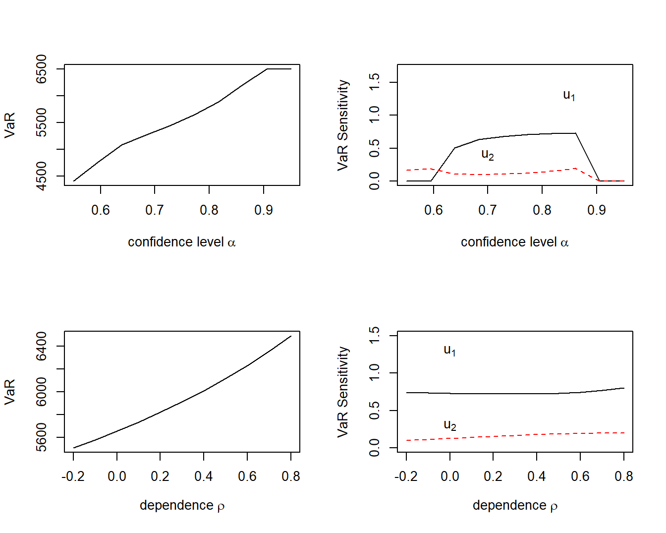
Example 5.6. Bivariate Excess of Loss VaR Sensitivities. Let us continue to use the distribution and parameter values from Example 5.3 and \(\alpha = 0.85\). As anticipated, from Figure 5.7 we see that the value at risk increases as both the confidence level \(\alpha\) increases (top left panel) and as the dependence parameter \(\rho\) increases (bottom left panel). The two right-hand panels show that both \(VaR\) sensitivities are positive for all values of \(\alpha\) and \(\rho\).
Expected Shortfall Sensitivities
The development of the \(ES\) sensitivity employs an auxiliary function that will also be useful for us in other contexts. To define this function, consider a generic random variable \(Y\) having distribution function \(F_Y\) with a unique \(\alpha\) quantile, \(F^{-1}(\alpha)\). Now, define the function
\[
ES1_F(z) = z + \frac{1}{1-\alpha} \left\{\mathrm{E}[Y] -\mathrm{E}[Y \wedge z]\right\} .
\]
From equation (2.3), one sees that the auxiliary function evaluated at the quantile is the expected shortfall, that is, \(ES(\alpha)=ES1_F(VaR_{\alpha})\).
After some calculations using this auxiliary function, one can show
\[\begin{equation}
\begin{array}{ll}
\partial_{\boldsymbol \theta} ~ES_{\alpha}[g(\mathbf{X};\theta)]
&=\frac{1}{1-\alpha} \left\{\partial_{\boldsymbol \theta}\mathrm{E}[g(X;\boldsymbol \theta)] -\left.\partial_{\boldsymbol \theta}\mathrm{E}[g(X;\boldsymbol \theta) \wedge y]\right|_{y=VaR(\boldsymbol \theta)}\right\} \\
&\ \ \ \ \ \ \ \ + \left( 1 - \frac{1}{1-\alpha} \{1-F[\boldsymbol \theta;VaR(\boldsymbol \theta)]\} \right)
\times \partial_{\boldsymbol \theta} VaR(\boldsymbol \theta).
\end{array}
\tag{5.7}
\end{equation}\]
Further,
\[\begin{equation}
\begin{array}{ll}
& \partial_{\boldsymbol \theta} \partial_{\boldsymbol \theta^{\prime}} ~ES_{\alpha}[g(\mathbf{X};\theta)] \\
&=
\frac{1}{1-\alpha} \left\{ \partial_{\boldsymbol \theta} \partial_{\boldsymbol \theta^{\prime}}\mathrm{E}[g(X;\boldsymbol \theta)] -\left. \partial_{\boldsymbol \theta} \partial_{\boldsymbol \theta^{\prime}}\mathrm{E}[g(X;\boldsymbol \theta) \wedge y]\right|_{y=VaR(\boldsymbol \theta)}\right\}\\
& \ \ \ \ \ \ \ + \left(1 - \frac{1}{1-\alpha} \{1-F[\boldsymbol \theta;VaR(\boldsymbol \theta)]\} \right)
\times \partial_{\boldsymbol \theta} \partial_{\boldsymbol \theta^{\prime}} VaR(\boldsymbol \theta) \\
& \ \ \ \ \ \ \ + \frac{1}{(1-\alpha)} F_y[\boldsymbol \theta,VaR(\boldsymbol \theta)] \times \partial_{\boldsymbol \theta}VaR(\boldsymbol \theta)
\times \partial_{\boldsymbol \theta^{\prime}} VaR(\boldsymbol \theta) .\\
\end{array}
\tag{5.8}
\end{equation}\]
Note that if \(VaR(\boldsymbol \theta)\) is a point of continuity (no discrete jump in the distribution function), then \(F[\boldsymbol \theta;VaR(\boldsymbol \theta)]= \alpha\). In this case, equations (5.7) and (5.8) become simpler. Specifically, the second term on the right-hand side of each equation becomes zero.
For the auxiliary function, define \(ES1_F(\boldsymbol \theta;y) = y + \frac{1}{1-\alpha} \left\{\mathrm{E}[g(X;\boldsymbol \theta)] -\mathrm{E}[g(X;\boldsymbol \theta) \wedge y]\right\}\).
Using equation (2.7), it is easy to see that \(\partial_y\mathrm{E}[g(X;\boldsymbol \theta) \wedge y] = 1-F(\boldsymbol \theta;y)\). Thus,
\[
\begin{array}{ll}
\partial_y ~ES1_F(\boldsymbol \theta;y) & = 1 - \frac{1}{1-\alpha} [1-F(\boldsymbol \theta;y)] .\\
\end{array}
\]
Now, with the other set of partial derivatives
\[
\begin{array}{ll}
\partial_{\boldsymbol \theta} ~ES1_F(\boldsymbol \theta;y) & = \frac{1}{1-\alpha} \left\{\partial_{\boldsymbol \theta}\mathrm{E}[g(X;\boldsymbol \theta)] -\partial_{\boldsymbol \theta}\mathrm{E}[g(X;\boldsymbol \theta) \wedge y]\right\} ,
\end{array}
\]
we can take differentials to yield
\[
{\small
\begin{array}{ll}
& \partial_{\boldsymbol \theta} ~ES_{\alpha}[g(\mathbf{X};\theta)] \\
&=
\partial_{\boldsymbol \theta} ~ES1_F[\boldsymbol \theta;VaR(\boldsymbol \theta)] \\
&= \left. \partial_{\boldsymbol \theta} ES1_F(\boldsymbol \theta;y) \right|_{y=VaR(\boldsymbol \theta)}
+ \left. \partial_{y} ES1_F(\boldsymbol \theta;y) \right|_{y=VaR(\boldsymbol \theta)}
\times \partial_{\boldsymbol \theta} VaR(\boldsymbol \theta) \\
&=\frac{1}{1-\alpha} \left\{\partial_{\boldsymbol \theta}\mathrm{E}[g(X;\boldsymbol \theta)] -\left.\partial_{\boldsymbol \theta}\mathrm{E}[g(X;\boldsymbol \theta) \wedge y]\right|_{y=VaR(\boldsymbol \theta)}\right\} \\
&\ \ \ \ \ \ \ \ + \left( 1 - \frac{1}{1-\alpha} \{1-F[\boldsymbol \theta;VaR(\boldsymbol \theta)]\} \right)
\times \partial_{\boldsymbol \theta} VaR(\boldsymbol \theta) ,
\end{array}
}
\]
as in equation (5.7).
Now consider partial second derivatives. First note that, because \(\partial_y\mathrm{E}[g(X;\boldsymbol \theta) \wedge y] = 1-F(\boldsymbol \theta;y)\), we have
\[
\begin{array}{ll}
\partial_y \partial_{\boldsymbol \theta}~\mathrm{E}[g(X;\boldsymbol \theta) \wedge y]
& = -\partial_{\boldsymbol \theta}F(\boldsymbol \theta;y) . \\
\end{array}
\]
With this, for the second term on the right hand side of equation (5.7), we have
\[
\begin{array}{ll}
\partial_{\boldsymbol \theta} &\left.\partial_{\boldsymbol \theta^{\prime}}\mathrm{E}[g(X;\boldsymbol \theta) \wedge y]\right|_{y=VaR(\boldsymbol \theta)}\\
&= \left.\partial_{\boldsymbol \theta}\partial_{\boldsymbol \theta^{\prime}}\mathrm{E}[g(X;\boldsymbol \theta) \wedge y]\right|_{y=VaR(\boldsymbol \theta)}\\
& \ \ \ \ \ \ \ +\left.\partial_y \partial_{\boldsymbol \theta}~\mathrm{E}[g(X;\boldsymbol \theta) \wedge y]\right|_{y=VaR(\boldsymbol \theta)}
\times \partial_{\boldsymbol \theta^{\prime}}VaR(\boldsymbol \theta)\\
&= \left.\partial_{\boldsymbol \theta}\partial_{\boldsymbol \theta^{\prime}}\mathrm{E}[g(X;\boldsymbol \theta) \wedge y]\right|_{y=VaR(\boldsymbol \theta)}\\
& \ \ \ \ \ \ \ - \left.\partial_{\boldsymbol \theta}F[\boldsymbol \theta;y]\right|_{y=VaR(\boldsymbol \theta)}
\times \partial_{\boldsymbol \theta^{\prime}}VaR(\boldsymbol \theta) .\\
\end{array}
\]
For the third term in equation (5.7),
\[
\begin{array}{ll}
\partial_{\boldsymbol \theta} & \left( 1 - \frac{1}{1-\alpha} \{1-F[\boldsymbol \theta;VaR(\boldsymbol \theta)]\} \right)
\times \partial_{\boldsymbol \theta^{\prime}} VaR(\boldsymbol \theta) \\
&= \left( 1 - \frac{1}{1-\alpha} \{1-F[\boldsymbol \theta;VaR(\boldsymbol \theta)]\} \right)
\times \partial_{\boldsymbol \theta} \partial_{\boldsymbol \theta^{\prime}} VaR(\boldsymbol \theta) \\
& \ \ \ \ \ + \left(\frac{1}{1-\alpha} \partial_{\boldsymbol \theta} F[\boldsymbol \theta,VaR(\boldsymbol \theta)]
\right) \times \partial_{\boldsymbol \theta^{\prime}} VaR(\boldsymbol \theta).
\end{array}
\]
Putting these together yields
\[
\begin{array}{ll}
& \partial_{\boldsymbol \theta} \partial_{\boldsymbol \theta^{\prime}} ~ES_{\alpha}[g(\mathbf{X};\theta)] \\
&= \frac{1}{1-\alpha} \left\{\partial_{\boldsymbol \theta}\partial_{\boldsymbol \theta^{\prime}}\mathrm{E}[g(X;\boldsymbol \theta)] -\left.\partial_{\boldsymbol \theta}\partial_{\boldsymbol \theta^{\prime}}\mathrm{E}[g(X;\boldsymbol \theta) \wedge y]\right|_{y=VaR(\boldsymbol \theta)}\right.\\
& \ \ \ \ \ \left. - ~\left.\partial_{\boldsymbol \theta}F[\boldsymbol \theta;y]\right|_{y=VaR(\boldsymbol \theta)}
\times \partial_{\boldsymbol \theta^{\prime}}VaR(\boldsymbol \theta) \right\} \\
& \ \ \ \ \ + \left(1 - \frac{1}{1-\alpha} \{1-F[\boldsymbol \theta;VaR(\boldsymbol \theta)]\} \right)
\times \partial_{\boldsymbol \theta} \partial_{\boldsymbol \theta^{\prime}} VaR(\boldsymbol \theta) \\
& \ \ \ \ \ + \frac{1}{1-\alpha} \partial_{\boldsymbol \theta} F[\boldsymbol \theta,VaR(\boldsymbol \theta)]
\times \partial_{\boldsymbol \theta^{\prime}} VaR(\boldsymbol \theta). \\
&= \frac{1}{1-\alpha} \left\{\partial_{\boldsymbol \theta}\partial_{\boldsymbol \theta^{\prime}}\mathrm{E}[g(X;\boldsymbol \theta)] -\left.\partial_{\boldsymbol \theta}\partial_{\boldsymbol \theta^{\prime}}\mathrm{E}[g(X;\boldsymbol \theta) \wedge y]\right|_{y=VaR(\boldsymbol \theta)}\right\}\\
& \ \ \ \ \ + \left(1 - \frac{1}{1-\alpha} \{1-F[\boldsymbol \theta;VaR(\boldsymbol \theta)]\} \right)
\times \partial_{\boldsymbol \theta} \partial_{\boldsymbol \theta^{\prime}} VaR(\boldsymbol \theta) \\
& \ \ \ \ \ + \frac{1}{1-\alpha} \left(\partial_{\boldsymbol \theta} F[\boldsymbol \theta,VaR(\boldsymbol \theta)] -
\left.\partial_{\boldsymbol \theta}F[\boldsymbol \theta;y]\right|_{y=VaR(\boldsymbol \theta)} \right)
\times \partial_{\boldsymbol \theta^{\prime}} VaR(\boldsymbol \theta)\\
&= \frac{1}{1-\alpha} \left\{\partial_{\boldsymbol \theta}\partial_{\boldsymbol \theta^{\prime}}\mathrm{E}[g(X;\boldsymbol \theta)] -\left.\partial_{\boldsymbol \theta}\partial_{\boldsymbol \theta^{\prime}}\mathrm{E}[g(X;\boldsymbol \theta) \wedge y]\right|_{y=VaR(\boldsymbol \theta)}\right\}\\
& \ \ \ \ \ + \left(1 - \frac{1}{1-\alpha} \{1-F[\boldsymbol \theta;VaR(\boldsymbol \theta)]\} \right)
\times \partial_{\boldsymbol \theta} \partial_{\boldsymbol \theta^{\prime}} VaR(\boldsymbol \theta) \\
& \ \ \ \ \ + \frac{1}{1-\alpha} F_y[\boldsymbol \theta,VaR(\boldsymbol \theta)] \times \partial_{\boldsymbol \theta}VaR(\boldsymbol \theta)
\times \partial_{\boldsymbol \theta^{\prime}} VaR(\boldsymbol \theta) ,\\
\end{array}
\]
where, in the last line, we recall that
\[
\partial_{\boldsymbol \theta} F[\boldsymbol \theta,VaR(\boldsymbol \theta)]
= F_{\boldsymbol \theta}[\boldsymbol \theta,VaR(\boldsymbol \theta)]
+ F_y[\boldsymbol \theta,VaR(\boldsymbol \theta)] \times \partial_{\boldsymbol \theta}VaR(\boldsymbol \theta).
\]
This is sufficient for equation (5.8).
Special Case. Two Risk Excess of Loss. As before, the vector of parameters is \(\boldsymbol \theta = (u_1,u_2)^{\prime}\) and the retained risk function is \(S(u_1,u_2)= X_1 \wedge u_1 + X_2 \wedge u_2\). In this case, we have
\[
\partial_{\boldsymbol \theta}\mathrm{E}[g(X;\boldsymbol \theta)] =
\left(\begin{array}{ll}
\partial_{u_1}\mathrm{E}[S(u_1,u_2)] \\
\partial_{u_2}\mathrm{E}[S(u_1,u_2)]
\end{array}\right)
= \left(\begin{array}{ll}
1-F_1(u_1) \\
1-F_2(u_2)
\end{array}\right)
\]
and
\[\begin{equation}
\partial_{\boldsymbol \theta}\mathrm{E}[g(X;\boldsymbol \theta)\wedge y] =
\left(\begin{array}{ll}
F_2(y-u_1) - C[F_1(u_1),F_2(y-u_1)] \\
F_1(y-u_2) - C[F_2(u_2),F_1(y-u_2)]
\end{array}\right) .
\tag{5.9}
\end{equation}\]
To see equation (5.9), we have the following.
\[
\begin{array}{ll}
\partial_{\boldsymbol \theta} \left\{\mathrm{E}[g(X;\boldsymbol \theta)\wedge y] \right\}
& = \partial_{\boldsymbol \theta} \left\{\int^y_{-\infty} [1-F(\boldsymbol \theta;z)]dz \right\} = -\int^y_{-\infty} ~F_{\boldsymbol \theta}(\boldsymbol \theta;z) dz .\\
\end{array}
\]
For the first retention parameter, using equation (5.2), we have
\[
\begin{array}{ll}
&\partial_{u_1} \left\{\mathrm{E}[g(X;\boldsymbol \theta)\wedge y] \right\} \\
& = -\int^y_{-\infty} ~F_{u_1}(u_1,u_2;z) dz \\
& = \int^y_{-\infty} ~f_2(z-u_1)\left\{1-C_2[F_1(u_1),F_2(z-u_1)] \right\} dz \\
& = F_2(y-u_1) - \int^y_{-\infty} ~\partial_z C[F_1(u_1),F_2(z-u_1)] dz \\
& = F_2(y-u_1) - C[F_1(u_1),F_2(y-u_1)] \\
& = \Pr(X_1 > u_1, X_2 \le y-u_1) .
\end{array}
\]
This is sufficient for equation (5.9).
Taking derivatives again yields
\[
\partial_{\boldsymbol \theta} \partial_{\boldsymbol \theta ^{\prime}} ~\mathrm{E}[g(X;\boldsymbol \theta)] =
- \left(\begin{array}{cc}
f_1(u_1) &0\\
0 & f_2(u_2)
\end{array}\right)
\]
and
\[
{\small
\begin{array}{ll}
\partial_{\boldsymbol \theta} \partial_{\boldsymbol \theta ^{\prime}} \mathrm{E}[g(X;\boldsymbol \theta)\wedge y] \\
\ \ \ =
\left(\begin{array}{cc}
f_2(y-u_1) \{1 - C_2[F_1(u_1),F_2(y-u_1)]\} & 0 \\
0& f_1(y-u_2)\{1 - C_2[F_2(u_2),F_1(y-u_2)] \}
\end{array}\right) .
\end{array}
}
\]
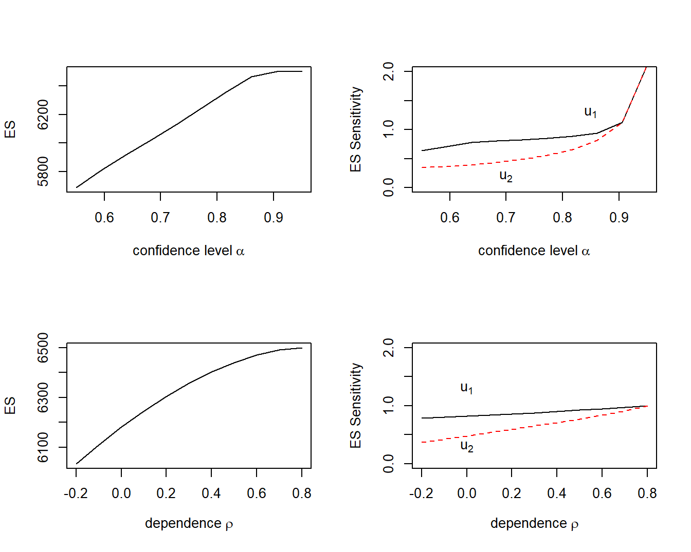
Example 5.7. Bivariate Excess of Loss - \(ES\) Sensitivities. We use the distribution and parameter values from Example 5.3 and \(\alpha = 0.85\). These yield interesting results in Figure 5.8.
Looking Forward. Sensitivity analysis will be the main theme of Chapters 9 and 10 so the foundations laid in this section will bear fruit for us later on. From this section’s detailed calculation of sensitivities, observe that the key aspect is the smoothness of parameters in potential outcomes of the retained risk and the retention parameters \(\boldsymbol \theta\). This smoothness is important and will motivate the introduction of kernel methods when we introduce simulation methods in Chapter 7.
Visualizing Constrained Optimization
Using constrained optimization, the goal is to find those parameter values \(u_1,u_2\) that minimizes an uncertainty measure of retained risk subject to the budget constraint that the risk transfer costs are limited by a given amount, \(RTC_{max}\). With the equation (3.3) structure, one can write this as
\[\begin{equation}
\boxed{
\begin{array}{lc}
{\small \text{minimize}_{u_1,u_2}} & ~~~~~RM[S(u_1, u_2)] \\
{\small \text{subject to}} & ~~~~~RTC(u_1, u_2) \le RTC_{max} \\
&u_1 \ge 0, \ \ \ \ u_2 \ge 0 .
\end{array}
}
\tag{5.10}
\end{equation}\]
This section introduces visualization techniques to help us understand the nuances of constrained optimization risk retention problems. As seen in Figure 5.4, it can be difficult to visualize a risk measure as a function of two upper limits. In addition, we want to get some insights by adding the budget constraint function that also could be represented as a three-dimensional figure (the constraint as a function of two upper limits). Instead, it is common in constrained optimization to utilize contours, a curve that is a function of two variables in which the function has a constant value.
Visualizing the Excess of Loss Problem
To explore visualization techniques, we start with \(ES\) minimization and then move on to \(VaR\) minimization. As will be demonstrated in Section 5.5, \(VaR\) minimization can be problematic.
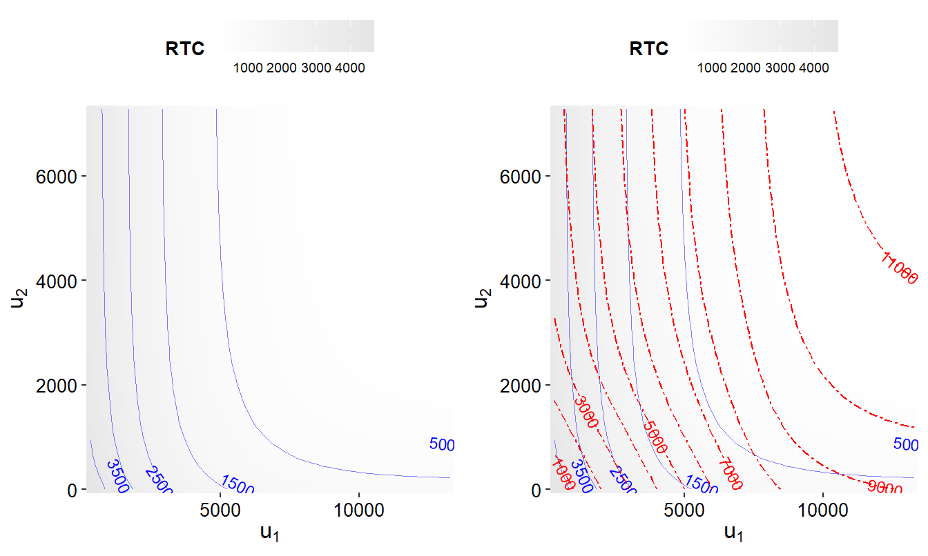
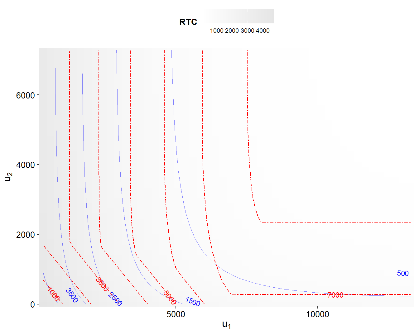
Example 5.8. Visualizing Excess of Loss Constrained Optimization - ES. Consider the distributions specified in Example 5.3, using a positive correlation \(\rho = 0.5\) and a confidence level \(\alpha = 0.85\). Figure 5.9 shows contours of the expected shortfall risk measure \(ES\) and the risk transfer cost \(RTC\) for several choices of upper limits \((u_1, u_2)\).
Specifically, the left-hand panel of Figure 5.9 shows the contours of the risk transfer cost \(RTC\) as solid blue curves. For this plot, darker shaded values indicate a larger value of \(RTC\). The contours are constant \(RTC\) slices as one might take in a three-dimensional graph such as Figure 5.4. For example, if \(RTC_{max} = 500\), then the feasibility region \(\{(u_1, u_2):RTC(u_1, u_2) \le 500\}\) corresponds to the area to the right and above the blue curve corresponding to \(RTC_{max} =500\).
The right-hand panel retains these contours with constant values of the expected shortfall \(ES\) superimposed as dashed red curves. For the optimization problem in Display (5.10), the objective is to find the smallest contour subject to being within this feasibility region. At the point of intersection where the smallest contour just meets the budget curve, the two curves are parallel.
# Example 5.8 Illustrative Code, Figure 5.9
# save(RMGridPos,
#      file = "../ChapTablesData/Chap5/Example521PosCorr.RData")
load( file = "ChapTablesData/Chap5/Example521PosCorr.RData")

ggRTC <- ggplot2::ggplot(RMGridPos, aes(x = u1, y = u2)) +
  geom_raster(aes(fill = RTC)) +
  geom_contour(aes(z = RTC), colour = FigBlue,
               size = 0.1, alpha = 0.5, bins = 6) +
  geom_text_contour(aes(z = RTC),  colour = FigBlue, size = 3) +
  labs(x = expression(u[1]),  y = expression(u[2]), fill = "RTC") +
  theme(legend.title = element_text(size = 10, face = "bold"),
  legend.position = "top", panel.background = element_blank(),
  axis.text = element_text(colour = "black", size = 10),
  axis.title = element_text(size = 12, face = "italic"),
  legend.text = element_text(size = 7),
  legend.key = element_blank() ) +
  scale_fill_continuous(low = "white", high = "grey90") +
  scale_y_continuous(expand = c(0,0) ) +
  scale_x_continuous(expand = c(0,0) )
ggPosCTE2 = ggRTC +
  geom_contour(aes(z = ES), colour = FigRed, linetype = 18) +
  geom_text_contour(aes(z = ES),  colour = FigRed , size = 3)
gridExtra::grid.arrange(ggRTC,ggPosCTE2,nrow=1)
# Example 5.9 Illustrative Code, Figure 5.10
ggPosVar2 = ggRTC +
  geom_contour(aes(z = VaR), colour = FigRed, linetype = 18) +
  geom_text_contour(aes(z = VaR),  colour = FigRed , size = 3)
ggPosVar2
To appreciate this visualization of the optimization problem, it is helpful to know where the optimal values lie when visualizing this graph. With \(RTC_{max} = 1,500\), when minimizing \(ES\), it turns out that the best values of the retention limits are \(u_1^* =3,379\) and \(u_2^* = 3,387\) with expected shortfall \(ES^* =5,997\). This allows one to identify this point in Figure 5.9.
Example 5.9. Visualizing Excess of Loss Constrained Optimization - VaR. Continuing from Example 5.8, we now consider the value at risk \(VaR\) risk measure. Figure 5.10 shows the \(RTC\) as solid blue curves and the \(VaR\) as dashed red curves. When the constraint is binding, the objective is to find the smallest contour subject to being at a given level of the risk transfer cost.
As before, it is helpful to know where the optimal values lie. It turns out that the best risk retention values are \(u_1^* =3,116\) and \(u_2^* =43,375\) (essentially infinity), resulting in a value at risk \(VaR^* =4,761\).
Similar calculations can be performed for other values of \(RTC_{max}\). For example, if \(RTC_{max} = 2,500\), it turns out that the best risk retention values are \(u_1^* =1,628\) and \(u_2^* =23,117\), resulting in a value at risk \(VaR^* =3,376\). As suggested by the graph, large changes in \(u_2\) mean only small changes in the optimal values of \(u_1\) and the \(VaR\), suggesting that they are not sensitive to \(u_2\).
From Figure 5.10, one sees that for this example we are able to determine the value of \(u_1\) well but determining a value of \(u_2\) is more problematic. When comparing this figure to the \(ES\) contour plot in Figure 5.10, it seems like the distinction between \(ES\) and \(RTC\) contours is more pronounced than the distinction between \(VaR\) and \(RTC\) contours, suggesting that it is easier to determine the optimal values for the \(ES\) problem.
Using Distribution Functions
When the risk measure is the value at risk (\(VaR\)), an equivalent problem formulation is
\[\begin{equation}
\boxed{
\begin{array}{lc}
{\small \text{minimize}_{u_1,u_2,x}} & ~~~~~x \\
{\small \text{subject to}} & ~~~~~\Pr[S(u_1, u_2) \le x] \ge \alpha \\
& ~~~~~RTC(u_1, u_2) \le RTC_{max} \\
&u_1 \ge 0, \ \ \ \ u_2 \ge 0 .
\end{array}
}
\tag{5.11}
\end{equation}\]
Intuitively, finding the smallest \(x\) value that minimizes the probability condition is equivalent to the quantile as described in Section 2.1. In this section, we simply provide code that solves each problem and show the equivalence between the two solutions. Section 7.2 will develop this general approach in a broader context, explaining its strengths and limitations compared to the basic approach, such as in Display (5.10).
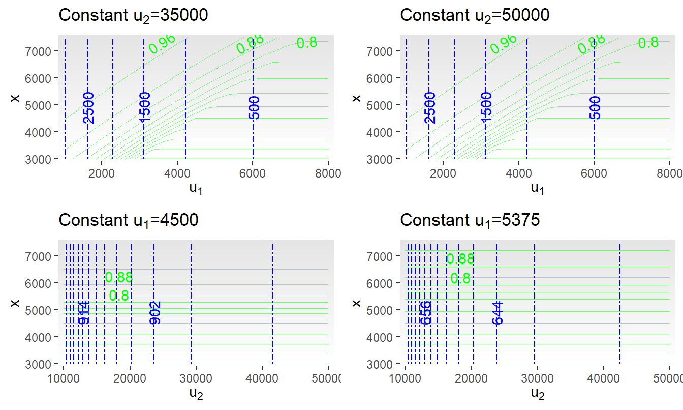
The minimization problem in Display (5.11) is complicated to visualize because now there are three decision variables, \(x\), \(u_1\), and \(u_2\), over which one seeks to evaluate the probability of the retained risk \(\Pr[S(u_1,u_2) \le x]\) and the risk transfer cost \(RTC\). Figure 5.11 shows different aspects of the problem; the top two panels hold the value of \(u_2\) as constant and the bottom two hold \(u_1\) constant. The upper left-hand panel is a contour plot of the probability of retained risk with the solid green curves representing the contours (the background shading is for values of \(x\)). As before, the dashed blue curves represent contours of the \(RTC\). For this panel, because we hold \(u_2=35,000\) fixed, the contour of \(RTC\) is simply a constant vertical line. The value of \(u_1 = 6,000\) corresponds to a risk transfer cost of \(RTC=500\). When \(x=7,000\), this vertical line is close to the contour corresponding to a probability value of 0.85. As we see below, these values turn out to give near optimal values.
There is little difference when comparing the top two panels of Figure 5.11. This is because the surface is relatively flat over different values of \(u_2\), meaning that changes in this variable have relatively little effect on the problem solution. The bottom two panels of Figure 5.11 each hold \(u_1\) constant. Here, in addition to vertical lines for the contours of \(RTC\), we see near horizontal lines for the contours of \(\Pr[S(u_1,u_2) \le x]\). This is additional evidence that changes in \(u_2\) have relatively little effect on the problem solution.
# Section 5.4.2, Figure 5.11

load( file = "ChapTablesData/Chap5/Sec542RMGridNoDFCorrB.RData")
lengthGrid = length(RMGridNoDF[,"u1"])
midpoint = RMGridNoDF[round(lengthGrid/2),]

RMGridNoDFmidu1A <- subset(RMGridNoDF, u1==as.numeric(midpoint["u1"]))
RMGridNoDFmidu1B <- subset(RMGridNoDF, u1==5375)
RMGridNoDFmidu2A <- subset(RMGridNoDF, u2==35000)
RMGridNoDFmidu2B <- subset(RMGridNoDF, u2==50000)
# str(RMGridNoDF)
# table(RMGridNoDF$u1)
# table(RMGridNoDF$u2)
breaksProb <- seq(0.80, 0.96, by = 0.04)
breaksRTC <- seq(200, 1200, by = 6)
ggNoDFConu1A = ggplot(RMGridNoDFmidu1A, aes(x = u2, y = x)) +
  geom_raster(aes(fill = x)) +
  geom_contour(aes(z = Prob), colour = FigGreen, size = 0.2, alpha = 0.5) +
  geom_text_contour(aes(z = Prob),  colour = FigGreen ,breaks = breaksProb) +
  geom_contour(aes(z = RTC), colour = FigBlue, linetype = 18) +
  geom_text_contour(aes(z = RTC),  colour = FigBlue ,breaks = breaksRTC) +
  theme(legend.position = "none") +
  scale_fill_continuous(low = "white", high = "grey90") +
  scale_y_continuous(expand = c(0,0)) +
  scale_x_continuous(expand = c(0,0)) +
  labs(x = expression(u[2]), title =expression(paste('Constant ', u[1], '=4500')))  #

ggNoDFConu1B = ggplot(RMGridNoDFmidu1B, aes(x = u2, y = x)) +
  geom_raster(aes(fill = x)) +
  geom_contour(aes(z = Prob), colour = FigGreen, size = 0.2, alpha = 0.5) +
  geom_text_contour(aes(z = Prob),  colour = FigGreen ,breaks = breaksProb) +
  geom_contour(aes(z = RTC), colour = FigBlue, linetype = 18) +
  geom_text_contour(aes(z = RTC),  colour = FigBlue ,breaks = breaksRTC) +
  theme(legend.position = "none") +
  scale_fill_continuous(low = "white", high = "grey90") +
  scale_y_continuous(expand = c(0,0)) +
  scale_x_continuous(expand = c(0,0)) +
  labs(x = expression(u[2]), title =expression(paste('Constant ', u[1], '=5375')))

ggNoDFConu2A = ggplot(RMGridNoDFmidu2A, aes(x = u1, y = x)) +
  geom_raster(aes(fill = x)) +
  geom_contour(aes(z = Prob), colour = FigGreen, size = 0.2, alpha = 0.5) +
  geom_text_contour(aes(z = Prob),  colour = FigGreen ,breaks = breaksProb) +
  geom_contour(aes(z = RTC), colour = FigBlue,linetype = 18) +
  geom_text_contour(aes(z = RTC),  colour = FigBlue ) +
  theme(legend.position = "none") +
  scale_fill_continuous(low = "white", high = "grey90") +
  scale_y_continuous(expand = c(0,0)) +
  scale_x_continuous(expand = c(0,0)) +
 labs(x = expression(u[1]), title =expression(paste('Constant ', u[2], '=35000')))

ggNoDFConu2B = ggplot(RMGridNoDFmidu2B, aes(x = u1, y = x)) +
  geom_raster(aes(fill = x)) +
  geom_contour(aes(z = Prob), colour = FigGreen, size = 0.2, alpha = 0.5) +
  geom_text_contour(aes(z = Prob),  colour = FigGreen ,breaks = breaksProb) +
  geom_contour(aes(z = RTC), colour = FigBlue, linetype = 18) +
  geom_text_contour(aes(z = RTC),  colour = FigBlue ) +
  theme(legend.position = "none") +
  scale_fill_continuous(low = "white", high = "grey90") +
  scale_y_continuous(expand = c(0,0)) +
  scale_x_continuous(expand = c(0,0)) +
  labs(x = expression(u[1]), title =expression(paste('Constant ', u[2], '=50000')))

gridExtra::grid.arrange(ggNoDFConu2A,ggNoDFConu2B,
             ggNoDFConu1A,ggNoDFConu1B, nrow=2)
To help interpret the figures, note that the optimal values of the problem in Display (5.11) are equivalent to those in Display (5.10). Interestingly the code for this alternative formulation (as in Display (5.11)) is much faster than for the code that optimizes directly the \(VaR\) risk measure. Intuitively, one can see in Figure 5.11 the sharp distinction among the contour curves. This is in contrast to the earlier Figure 5.9 where the near parallel contours suggested difficulties in the algorithms arriving at optimal solutions.
Restricting the Feasible Region
As in Display (5.10), we seek to solve the problem
\[
\boxed{
\begin{array}{lc}
{\small \text{minimize}_{u_1,u_2}} & ~~~~~RM[S(u_1, u_2)] \\
{\small \text{subject to}} & ~~~~~RTC(u_1, u_2) \le RTC_{max} \\
&u_1 \ge 0, \ \ \ \ u_2 \ge 0 .
\end{array}
}
\]
The feasible region is within the quadrant where values of \(u_1\) and \(u_2\) are non-negative. Moreover, there is an additional restriction in the budget constraint, \(RTC(u_1, u_2) \le RTC_{max}\). As will be seen, for small values of \(RTC_{max}\) this restriction can be considerable. By recognizing in advance the restrictions on the feasible region, optimization algorithms will have a smaller region to search over which to optimize, potentially improving their convergence.
As a tactic for reducing the feasible region, one might look to solutions where one selects parameter values so that transfer costs are at the maximum, that is, values of \(u_1\) and \(u_2\) so that \(RTC(u_1, u_2) = RTC_{max}\). In addition, analysts are sometimes simply given an equality constraint, “this is what you spend.” You will recall that this choice results in an active, or binding, constraint.
By restricting ourselves to feasible sets where the constraint is binding, we have reduced the number of “free” decision variables by one. This can be especially useful in the case of two risks with upper limits where there are only two decision variables; with a binding constraint, we have reduced the dimension of the problem to a single variable. That is, if a value of \(u_1\) is known, then subject to mild regularity conditions, we can solve for the value of \(u_2\) through the equation \(RTC(u_1, u_2) = RTC_{max}\). However, this tactic comes with caveats; it is also well known in the optimization literature (see for example, Nocedal and Wright (2006), Section 15.3) that this approach can introduce some subtle errors into the problem formulation. As summarized by Nocedal and Wright (2006), “Elimination techniques must be used with care, however, as they may alter the problem or introduce ill conditioning.”
Budget Restriction
As introduced in Section 3.2, the risk transfer cost \(RTC\) is the expense associated with offloading risks. You can think of limiting the \(RTC\) by a fixed amount, \(RTC_{max}\), as our budget restriction. As with all constrained optimization problems, imposing a constraint can restrict the feasible set of candidate parameter values.
To develop intuition, we make two simplifying assumptions. First, let us focus on risk transfer costs that are additive so that we may write \(RTC(u_1,u_2)\) \(= RC_1(u_1)\) \(+ RC_2(u_2)\), where \(RC_j(u)\) is the risk transfer cost for the \(j\)th risk, \(j=1,2\). As will be discussed in Section 7.5.1, this is a very natural assumption to make with separate risk transfer agreements.
Second, consider “fair” risk costs of the form \(RC_j(u) = \int^{\infty}_u [1-F_j(x)]dx\) for \(j=1,2\), as in equation (3.4). It is easy to extend this fair risk cost using multiplicative constants to allow for administrative expenses. Alternatively, risk managers may prefer to use measures such as quantiles for risk costs instead of expectations.
Guidelines for Setting the Maximal Risk Transfer Cost
We first look to bounds on the \(RTC\) function to guide setting the maximal cost \(RTC_{max}\). For example, if \(RTC_{max}\) is greater than the upper bound of the function \(RTC\) then the constraint does not impose any limitations on the minimization problem and one can ignore the constraint. In the same way, if \(RTC_{max}\) is less than the lower bound of the \(RTC\) function, then there are no feasible parameter values for the optimization problem.
With additive fair risk transfer costs, we have
\[\begin{equation}
\begin{array}{ll}
RTC[u_1,u_2] &= RC_1(u_1) +RC_2(u_2) \\
&= \int^{\infty}_{u_1} [1-F_1(x)]~dx + \int^{\infty}_{u_2} [1-F_2(x)]~dx .
\end{array}
\tag{5.12}
\end{equation}\]
This \(RTC\) is bounded by
\[
\begin{array}{ll}
0 = RTC[\infty,\infty] &\le RTC[u_1,u_2] \\ &
\le RTC[0,0] = \mathrm{E}(X_1)+\mathrm{E}(X_2).
\end{array}
\]
Thus, we only consider values of maximal cost \(RTC_{max}\) such that \(0 < RTC_{max}\) \(< \mathrm{E}(X_1)+\mathrm{E}(X_2)\), so that the constraint has some meaning.
In addition, sometimes one wants to know about bounds on the \(RTC\) function when there are restrictions on one of the parameters. For example, suppose that \(u_2=0\), meaning that all of the risk \(X_2\) is transferred (nothing is retained). Then, the bounds on the \(RTC\) function over different choices of \(u_1\) are
\[
\mathrm{E}(X_2) = RTC[\infty,0] \le RTC[u_1,0] \le RTC[0,0] = \mathrm{E}(X_1)+\mathrm{E}(X_2).
\]
Thus, when \(u_2=0\), a selection of \(RTC_{max} < \mathrm{E}(X_2)\) means that the feasible set is null so that the problem is not well defined. Table 5.1 summarizes this and additional bounds.
Table 5.1. Bounds on the Fair Risk Transfer Cost Function
\[
\begin{array}{c|cc}\hline
\text{Known} & \text{Lower Bound} & \text{Upper Bound} \\
\text{Parameter Values} & & \\\hline
u_1=0 & \mathrm{E}(X_1)& \mathrm{E}(X_1)+\mathrm{E}(X_2)\\
u_1=\infty & 0 & \mathrm{E}(X_2) \\
u_2=0 & \mathrm{E}(X_2)& \mathrm{E}(X_1)+\mathrm{E}(X_2)\\
u_2=\infty & 0 &\mathrm{E}(X_1) \\ \hline
\end{array}
\]
As a consequence, suppose that one sets the maximal transfer cost so that \(RTC_{max} < \min \{\mathrm{E}(X_1), \mathrm{E}(X_2)\}\). Then, on the feasible set where \(RTC(u_1,u_2) \le RTC_{max}\), both \(u_1\) and \(u_2\) are positive.
Table 5.1: Silly. Create a table just to update the counter…
| 2 |
Limitations on Risk Retention Parameters Imposed by Constraints
For the feasible set, we require \(u_1 \ge 0,u_2 \ge 0\) and \(0 \le RC_1(u_1) + RC_2(u_2) \le RTC_{max}\). This means that \(RC_j(u_j) \le RTC_{max}\) that we can also write as \(u_j \ge RC_j^{-1}[RTC_{max}]\), for \(j=1,2\). Here, \(RC_j^{-1}\) is the inverse of the cost function \(RC_j\) that may be defined as \(RC_j^{-1}(t) = \inf\{u: RC_j(u) \le t \}\). Thus, if the maximal risk transfer cost is sufficiently small, then we can get some information about the lower bounds for the risk retention parameters \(u_1, u_2\). This is illustrated in the following example.
Example 5.10. Parameter Limits for Gamma and Pareto Distributions. Let \(X_1\) have a gamma distribution with shape parameter 2 and scale parameter 2,000 and let \(X_2\) have a Pareto distribution with shape parameter 3 and scale parameter 2,000. Their relationship is governed by a normal copula with parameter \(\rho = 0.5\). For demonstration purposes, we assume a maximal risk transfer cost is 0.30 times the sum of expected losses. With \(\mathrm{E}(X_1) =\) 4,000, \(\mathrm{E}(X_2) =\) 1,000, this means that \(RTC_{max} =\) 1,500.
# Example 5.10 Illustrative Code, Part A
RTCmax <- 0.30*(ERisk1fun() + ERisk2fun())
alpha <- 0.85
# Lower/Upper Bounds for Active Trade-off Function AT

Ubdd.fct <- function(j, RTCmax){
  RCj          <- function(u){RC1(u)*(j==1) + RC2(u)*(j==2)}
  Excess       <- RTCmax - (RTC(0,0) - RCj(0))
  Ubdd.AT.fctj <- function(u){Excess - RCj(u)}
  Upperbdd     <- 1.0e8
  if (Excess > 0) {Upperbdd <-
          uniroot(Ubdd.AT.fctj, lower = 0, upper =5e4)$root}
  return(Upperbdd)
  }
Lbdd.fct <- function(j, RTCmax){
  RCj          <- function(u){RC1(u)*(j==1) + RC2(u)*(j==2)}
  Lbdd.AT.fctj <- function(u){RTCmax - RCj(u)}
  Lowerbdd     <- 0
  if (RTCmax < RCj(0) ) {Lowerbdd <-
          uniroot(Lbdd.AT.fctj, lower = 0, upper = 5e4)$root}
  return(Lowerbdd)
  }
ATj.fct  <- function(j,u, RTCmax){
  RCj    <- function(u){RC1(u)*(j==1) + RC2(u)*(j==2)}
  RCnej  <- function(u){RC1(u)*(j != 1) + RC2(u)*(j != 2)}
  RCnejx <- function(x){RTCmax - RCj(u) - RCnej(x)}
  ustar  <- 1.0e8
  if (RTCmax - RCj(u) >= RCnej(0) ) {ustar <- 0}
  if ( (RTCmax - RCj(u) > 0)*(RTCmax - RCj(u) < RCnej(0)) ) {
           ustar <- uniroot(RCnejx, lower =  0, upper =1e9)$root}
  return(ustar)
  }
AT1.fct <- function(u1,RTCmax){
  RC2x   <- function(x){RTCmax - RC1(u1) - RC2(x)}
  u2star <- 1.0e8 #1.2e4
  if ( RTCmax - RC1(u1) >= RC2(0) ) {u2star <- 0}
  if ( (RTCmax - RC1(u1) > 0)*(RTCmax - RC1(u1) < RC2(0)) ) {
          u2star <- uniroot(RC2x, lower =  0, upper =1e9)$root}
  return(u2star)
}
# Example 5.10 Illustrative Code, Part B
OutMat.U    <- matrix(0,nrow = 8, ncol = 2)
u1.u1Lower  <- Lbdd.fct(1, RTCmax)+0.001-> OutMat.U[1,1]
u2.u1Lower  <- ATj.fct(1,u1.u1Lower, RTCmax) -> OutMat.U[2,1]
tempLower   <- ExLossESGamPareto(u1.u1Lower,u2.u1Lower,rho,alpha)
VaR.u1Lower <- tempLower[[2]]         -> OutMat.U[3,1]
CTE.u1Lower <- tempLower[[3]]         -> OutMat.U[4,1]
u1.u1Upper  <- Ubdd.fct(1, RTCmax)    -> OutMat.U[5,1]
u2.u1Upper  <- ATj.fct(1,u1.u1Upper, RTCmax) -> OutMat.U[6,1]
tempUpper   <- ExLossESGamPareto(u1.u1Upper,u2.u1Upper,rho,alpha)
VaR.u1Upper <- tempUpper[[2]]         -> OutMat.U[7,1]
CTE.u1Upper <- tempUpper[[3]]         -> OutMat.U[8,1]

u2.u2Lower  <- Lbdd.fct(2, RTCmax)+0.00-> OutMat.U[2,2]
u1.u2Lower  <- ATj.fct(2,u2.u2Lower, RTCmax) -> OutMat.U[1,2]
tempLower   <- ExLossESGamPareto(u1.u2Lower,u2.u2Lower,rho,alpha)
VaR.u2Lower <- tempLower[[2]]          -> OutMat.U[3,2]
CTE.u2Lower <- tempLower[[3]]          -> OutMat.U[4,2]
u2.u2Upper  <- Ubdd.fct(2, RTCmax)     -> OutMat.U[6,2]
u1.u2Upper  <- ATj.fct(2,u2.u2Upper, RTCmax) -> OutMat.U[5,2]
tempUpper   <- ExLossESGamPareto(u1.u2Upper,u2.u2Upper,rho,alpha)
VaR.u2Upper <- tempUpper[[2]]          -> OutMat.U[7,2]
CTE.u2Upper <- tempUpper[[3]]          -> OutMat.U[8,2]

save(OutMat.U,
     file = "../ChapTablesData/Chap5/Ex551ActiveConstraints.RData")
For this example, it turns out that the lower bound for \(u_1\) is \(RC^{-1}_1(1500) =\) 3,113 and the lower bound for \(u_2\) is 0. Because the maximal risk transfer cost exceeds the expected risk, \(RTC_{max} > \mathrm{E}(X_2)\), it seems reasonable that there is no additional information about the lower bound for \(u_2\).
Active Constraint Feasible Region
It is natural to test limiting values so that one approaches the point where a constraint becomes active in the sense that \(RTC(u_1,u_2) = RTC_{max}\). How does the choice of \(RTC_{max}\) affect the set of risk retention parameters that achieve an active constraint? These parameter bounds could also provide useful starting values for the broader constrained optimization problem (where we do not impose an active constraint in advance).
Let us now consider limitations on the feasible set imposed by the active budget constraint \(RTC(u_1,u_2) = RTC_{max}\). With \(RC_1(u_1) + RC_2(u_2)=RTC_{max}\), we define
\[\begin{equation}
AT_{1,RC}(u_1) = RC_2^{-1}[RTC_{max} - RC_1(u_1)] = u_2,
\tag{5.13}
\end{equation}\]
a trade-off function among parameter values at the active constraint. The requirement that \(0 \le u_2 \le \infty\) implies constraints on \(u_1\) in that
\[\begin{equation}
\max\left[0,RTC_{max}- RC_2(0) \right] \le RC_1(u_1) \le RTC_{max} .
\tag{5.14}
\end{equation}\]
Starting with \(0 \le u_2 \le \infty\), we have
\[
\begin{array}{lc}
&0 \le AT_{1,RC}(u_1) = RC_2^{-1}[RTC_{max} - RC_1(u_1)] \le \infty \\
\iff &
0 =RC_2(\infty) \le RTC_{max} - RC_1(u_1) \le RC_2(0) \\
\iff & - RC_2(0) \le RC_1(u_1) - RTC_{max} \le 0 \\
\iff& RTC_{max}- RC_2(0) \le RC_1(u_1) \le RTC_{max} .\\
\end{array}
\]
In the case that \(RTC_{max} < RC_2(0)\), we can use 0 as a lower bound on \(RC_1(u_1)\). This is sufficient for equation (5.14).
To see this result, consider the following minimal scenario.
Example 5.11. Fair Transfer Costs, Uniform Distributions. Assume that \(X_1, X_2\) are both uniformly distributed on [0,1]. From equation (5.12), we have \(RC_j(u) = (1-u)^2/2\) and so \(RC_j^{-1}(y) = 1- \sqrt{2y}\). With this and equation (5.14), we have
\[
\max \left[0 , RTC_{max}- \frac{1}{2} \right] \le \frac{(1-u_1)^2}{2} \le RTC_{max} .
\]
This is equivalent to
\[
\max[0, 1-\sqrt{2 RTC_{max}} \ ] \le u_1 \le 1 - \sqrt{\max[0 , (2RTC_{max}-1)]} \ \ \ .
\]
Values of \(u_1\) outside of the boundaries may represent legitimate risk parameters but cannot achieve an active constraint.
For valid values of \(u_1\), from equation (5.13), we have
\[
AT_{1,RC}(u_1) = 1 - \sqrt{2 RTC_{max} - (1-u_1)^2} ~,
\]
for the trade-off function. Figure 5.12 shows this trade-off function with these bounds. Note that values of \(u_1\) or \(u_2\) at zero signify total risk transfer and values at one signify total risk retention.
# Example 5.11 Illustrative Code, Figure 5.12
ATUnif <- function(u,RTCmax){
  sqroot = 2*RTCmax-(1-u)**2
  Gu <- 1-sqrt(sqroot*(sqroot>0))
  Gu <- Gu*(Gu>0)
  Gu <- pmin(1,Gu)
  return(Gu)
  }
uparambase<- seq(0, 1, length.out = 110)
u.0.4 <- ATUnif(uparambase, RTCmax = 0.4)
u.0.5 <- ATUnif(uparambase, RTCmax = 0.5)
u.0.2 <- ATUnif(uparambase, RTCmax = 0.2)
u.0.8 <- ATUnif(uparambase, RTCmax = 0.8)
RTCmax = 0.8
plot(uparambase,u.0.8, type = "l", lty = 1,
     xlab = "u", ylab = "AT(u)", ylim=c(0,1) )
  lines(uparambase,u.0.5, lty = 2, col = FigRed)
  lines(uparambase,u.0.4, lty = 3, col = FigBlue)
  lines(uparambase,u.0.2, lty = 4, col = FigGreen)
Limitations on Risk Retention Parameters Imposed by an Active Constraint
For an active constraint, \((u_1,u_2)\) are such that \(RC_1(u_1) + RC_2(u_2) = RTC_{max}\) and so there is only one free parameter, bring us back to the discussion in Section 5.5.1 with a known parameter. Formally, given \(u_1\), one can determine \(u_2\) through the active trade-off function in equation (5.13). In the same way, we can define a second active trade-off function
\[
\begin{array}{lc}
AT_{2,RC}(u_2) = RC_1^{-1}[RTC_{max} - RC_2(u_2)] = u_1 .\\
\end{array}
\]
that provides an expression to determine \(u_1\) based on knowledge of \(u_2\).
From equation (5.14), we can define two feasible sets:
\[
\begin{array}{ll}
FS_1 = \{u_1 \ge 0:\max\{0,RTC_{max}- RC_2(0) \} \le RC_1(u_1) \le RTC_{max} \} \\
FS_2 = \{u_2 \ge 0:\max\{0,RTC_{max}- RC_1(0) \} \le RC_2(u_2) \le RTC_{max} \} &. \\
\end{array}
\]
- Assuming that the constraint is binding or active, we can also get an upper bound on each parameter (that may be infinity).
- The upper bound for \(u_1\) comes from the inequality \(\max\{0,RTC_{max}- RC_2(0) \} \le RC_1(u_1)\) and similarly for \(u_2\).
- Note that these feasible sets depend on the maximal risk transfer cost, \(RTC_{max}\).
Example 5.12. Active Constraint Parameter Limitations. Table 5.2 provides these bounds using the assumptions of Example 5.10. Using equation (5.14) and \(FS_1\), we can determine a lower bound imposed by the active constraint limitation on \(u_1\) as \(u_{1,lower} = RC_1^{-1}(RTC_{max}) = 3,113\). With the value of \(u_{1,lower}\), we can compute the corresponding value for \(u_2=AT_{1,RC}(u_{1,lower}) =2,717,751\) (that is essentially infinity), as well as the \(VaR =4,757\) and \(ES =6,674\).
Because \(RTC_{max} > \mathrm{E}(X_2) = RC_2(0)\), we also have a finite upper bound on \(u_1\). This is \(u_{1,upper} = RC_1^{-1}[RTC_{max}- RC_2(0)] =5,989\). To summarize, from the table we see that the set of bounds on \(u_1\) for the first feasible set \(FS_1\) is [3113, 5989]. In the same way, the set of bounds on \(u_2\) for the second feasible set \(FS_2\) is [0.00, 100000000], meaning that essentially no bounds are available for this parameter.
Table 5.2: Bounds and Risk Measures
|
|
Feasible Set 1
|
Feasible Set 2
|
|
\(u_1\) Based on Lower \(u\) in the FS
|
3113
|
5989
|
|
\(u_2\) Based on Lower \(u\) in the FS
|
2717751
|
0
|
|
\(VaR\) Based on Lower \(u\) in the FS
|
4231
|
5989
|
|
\(ES\) Based on Lower \(u\) in the FS
|
5809
|
5989
|
|
\(u_1\) Based on Upper \(u\) in the FS
|
5989
|
3113
|
|
\(u_2\) Based on Upper \(u\) in the FS
|
0
|
100000000
|
|
\(VaR\) Based on Upper \(u\) in the FS
|
5989
|
4231
|
|
\(ES\) Based on Upper \(u\) in the FS
|
5989
|
5809
|
Active Constraint Objective Function
By working with feasible sets limited by the active constraint, we can replace the problem summarized in Display (5.10) with
\[\begin{equation}
\boxed{
\begin{array}{lc}
{\small \text{minimize}_{u_1}} & ~~~~~RM[S(u_1, AT_{1,RC}(u_1))] ,\\
{\small \text{subject to}} &\max\{0,RTC_{max}- RC_2(0) \} \le RC_1(u_1) \le RTC_{max} \\
& u_1 \ge 0.
\end{array}
}
\tag{5.15}
\end{equation}\]
This uses the active trade-off function \(AT_{1,RC}(u)\) defined in equation (5.13). Although certainly less intuitive, it is only a one-parameter problem. We could also express Display (5.15) in terms of the second trade-off function \(AT_{2,RC}\) and feasible set \(FS_2\). Although in principle they have the same solutions, the choice can matter in terms of numerical stability.
This section demonstrates, as suggested by Nocedal and Wright (2006), that the objective function varying over this restricted region can exhibit unanticipated behavior.
To start, we now return to Example 5.11 where the risks have identical distributions. In this case, the two functions are the same. The point of this illustration is to emphasize the importance of the dependence between risks.
Example 5.13. Visualizing the Objective Function, Uniform Distributions. Extending Example 5.11, we now assume the maximal risk transfer cost is \(RTC_{max} = 0.2\). With this, the parameter bounds become
\[
\begin{array}{ll}
0.3675 & \approx 1-\sqrt{0.4} \\
& = \max[0, 1-\sqrt{2 RTC_{max}} \ ] \le u_1 \le 1 - \sqrt{\max[0 , (2RTC_{max}-1)]} = 1 .
\end{array}
\]
From \(RC(u) = (1-u)^2/2\), one can easily verify that the inverse function is \(RC^{-1}(y) = 1 - \sqrt{2y}\). Thus, with equation (5.13), we have the active trade-off function to be
\[
\begin{array}{ll}
AT_{RC}(u) = RC^{-1}[RTC_{max} - RC(u)] =1 - \sqrt {0.4 - (1-u)^2} .\\
\end{array}
\]
Figure 5.13 summarizes results; it is a remarkable figure. This figure suggests that the optimization problem depends in a critical way on the dependence, reinforcing observations made in Example 5.2.
- The left-hand panel suggests that the \(VaR\) does not depend on \(u_1\) at the solid black line corresponding to the case of independence. The dotted red curve is for a negative Spearman correlation -0.5, the dashed blue curve is for a positive correlation 0.5 (I use confidence level \(\alpha = 0.7\) for this graph). For negatively dependent risks marked by the dashed red curve, an analyst could use a standard optimization technique, such as seeking a point where the gradient is zero, to determine the best value of \(u\) to minimize the \(VaR\). However, if one uses the same technique for positive dependent risks remarked by the dotted blue curve, the “best” value of \(u\) results in the maximum \(VaR\). The solid black line is flat, suggesting that the analyst would find this optimization problem to be challenging.
- The right-hand panel shows the relation between the upper limit and the \(ES\). This figure is more comforting in that, regardless of the dependence, one could use a standard optimization technique to determine its minimal value. Less comforting is the fact that one could get a very different optimal point, depending on whether one uses the \(VaR\) or \(ES\) as the risk measure.
# Example 5.13 Illustrative Code
RCUnif  <- function(u){ 0.5 - (1-u)**2/2 }
RTCstar <- function(u1,u2,RTCmax){ RCUnif(u1) + RCUnif(u2) - RTCmax }

ATUnif <- function(u,RTCmax){
  sqroot <- 2*RTCmax-(1-u)**2
  Gu <- 1-sqrt(sqroot*(sqroot>0))
  Gu <- Gu*(Gu>0)
  Gu <- pmin(1,Gu)
  return(Gu)
  }
ExLossCTEUnif <- function(u1,u2,rho,alpha){
    Prob.alpha      <- function(y){Prob.fct(u1,u2,rho,y) - alpha}
    VaR             <- uniroot(Prob.alpha, lower = 0, upper = 10e6)$root
    Surv.fct.y      <- function(y){1-Prob.fct(u1,u2,rho,y)}
    Surv.fct.y.vec  <- Vectorize(Surv.fct.y)
    Sum.limited.Var <-  integrate(Surv.fct.y.vec, lower = 0, upper = VaR)$value
    TotalRetained   <- u1-u1**2/2 + u2-u2**2/2
    CTE             <- VaR + (TotalRetained- Sum.limited.Var)/(1-alpha)
    Output          <- list(Prob.fct(u1,u2,rho,y=1.1),VaR,CTE)
    return(Output)
    }
RTCmax    <- 0.2
alpha     <- 0.7
u1base    <- seq(0.4, 0.9, length.out = 10) -> u2gen
for (iparam in 1:length(u1base)) {
       u2gen[iparam] = ATUnif(u1base[iparam], RTCmax) }
Prob.mat <- matrix(0,3,length(u1base))
VaR.mat  <- matrix(0,3,length(u1base))
CTE.mat  <- matrix(0,3,length(u1base))

for (iparam in 1:length(u1base)) {
  T1   <- ExLossCTEUnif(u1=u1base[iparam],u2=u2gen[iparam], rho=-0.5,alpha)
  Prob.mat[1,iparam] <- T1[[1]]
  VaR.mat[1,iparam]  <- T1[[2]]
  CTE.mat[1,iparam]  <- T1[[3]]
  T1 <- ExLossCTEUnif(u1=u1base[iparam],u2=u2gen[iparam], rho= 0.000001,alpha)
  Prob.mat[2,iparam] <- T1[[1]]
  VaR.mat[2,iparam]  <- T1[[2]]
  CTE.mat[2,iparam]  <- T1[[3]]
  T1 <- ExLossCTEUnif(u1=u1base[iparam],u2=u2gen[iparam], rho= 0.5,alpha)
  Prob.mat[3,iparam] <- T1[[1]]
  VaR.mat[3,iparam]  <- T1[[2]]
  CTE.mat[3,iparam]  <- T1[[3]]
  }

save(u1base,VaR.mat,CTE.mat,
     file = "../ChapTablesData/Chap5/Ex552FairCostsUniform.RData")
# Example 5.13 Illustrative Code, Figure 5.13
# save(u1base,VaR.mat,CTE.mat,
#      file = "../ChapTablesData/Chap5/Ex552FairCostsUniform.RData")
load( file = "ChapTablesData/Chap5/Ex552FairCostsUniform.RData")

par(mfrow = c(1,2))
  plot(u1base,VaR.mat[2,], type = "l", lty = 1,
       xlab = expression(u[1]), ylab = "VaR", ylim=c(0.90,1.1))
    lines(u1base,VaR.mat[1,],  col=FigRed, lty=3)
    lines(u1base,VaR.mat[3,],  col=FigBlue, lty=2)
  plot(u1base,CTE.mat[2,], type = "l", lty = 1,
       xlab = expression(u[1]), ylab = "ES", ylim=c(1,1.2))
    lines(u1base,CTE.mat[1,],  col=FigRed, lty=3)
    lines(u1base,CTE.mat[3,],  col=FigBlue, lty=2)
This example underscores the importance of dependence between risks, a topic that we take up in Chapter 12.
Example 5.14. Visualizing the Objective Function with an Active Constraint. The observations from Example 5.11 are not unique to the uniform distribution. To verify this, we return to the set-up in Example 5.12. Figure 5.14 shows the value at risk and the expected shortfall for \(u_1\) in the interval \([u_{1,lower}, u_{1,upper}]\).
# Example 5.14 Illustrative Code
# Lower/Upper Bounds for Active Trade-off Function AT

AT.fct <- function(u1,RTCmax){
  RC2x <- function(x){RTCmax - RC1(u1) - RC2(x)}
  u2star <- 1.0e8 #1.2e4
  if (RTCmax - RC1(u1) >= RC2(0)) {u2star <- 0}
  if ((RTCmax - RC1(u1) > 0)*(RTCmax - RC1(u1) < RC2(0))) {
       u2star <- uniroot(RC2x, lower =  0, upper =1e9)$root}
  return(u2star)
}

ATu.fct <- function(u1){AT.fct(u1,RTCmax=RTCmax)}

f0.VaRu <- function(u1) {
  u2=ATu.fct(u1)
  Prob.alpha <- function(y){3e5*(Prob.fct(u1,u2,rho,y) - alpha)}
  VaR <- uniroot(Prob.alpha, lower = 0, upper = 5e4)$root
  return(VaR)
  }
f0.CTEu <- function(u1) {
  u2=ATu.fct(u1)
  Prob.alpha <- function(y){Prob.fct(u1,u2,rho,y) - alpha}
  VaR <- uniroot(Prob.alpha, lower = 0, upper = 5e4)$root
  Surv.fct.y <- function(y){1-Prob.fct(u1,u2,rho,y)}
  Surv.fct.y.vec <- Vectorize(Surv.fct.y)
  Sum.limited.Var <- integrate(Surv.fct.y.vec, lower = 0, upper = VaR)$value
  TotalRetained <-
      actuar::levgamma(limit = u1,shape = risk1shape, scale = risk1scale) +
      actuar::levpareto(limit = u2,shape = risk2shape, scale = risk2scale)
    CTE <- VaR + (TotalRetained- Sum.limited.Var)/(1-alpha)
  return(CTE)
  }
From the left-hand panel of Figure 5.14, we see that \(u_1=u_{1,lower}\) minimizes the value at risk. A numerical optimization routine that searches for a stationary point (with a zero derivative) will have difficulty reaching this conclusion. In contrast, from the right-hand panel, minimization of the expected shortfall can readily be accomplished with numerical optimization routines. The associated code demonstrates how to use the R function optimize. It verifies that, minimizing \(VaR\), the best value of \(u_1\) is 3,113 with value at risk \(VaR^* =\) 4,757 and expected shortfall \(ES^* =\) 6,673. Further, minimizing \(ES\), the best value of \(u_1\) is 4,257 with value at risk \(VaR^* =\) 5,038 and expected shortfall \(ES^* =\) 5,038.
# Example514A
Ubdd.AT.fct <- function(u){RTCmax - RC2(0) - RC1(u)}
Upperbdd    <- 1.0e5
if (RTCmax - RC2(0) > 0) {
       Upperbdd <- uniroot(Ubdd.AT.fct, lower = 0, upper =1e6)$root}
Lbdd.AT.fct <- function(u){RTCmax - RC1(u)}
Lowerbdd    <- uniroot(Lbdd.AT.fct, lower = 0, upper =1e6)$root
u1opt       <- optimize(f0.VaRu, interval = c(Lowerbdd, 4000), tol = 0.1)
u1opt2      <- optimize(f0.CTEu, interval = c(Lowerbdd, Upperbdd), tol = 0.1)

u1VaRopt.1    <- round(u1opt$minimum,digits=2)
u2VaRopt.1    <- round(AT.fct(u1=u1VaRopt.1+.001,RTCmax),digits=2)
VaRu1VaRopt.1 <- round(ExLossESGamPareto(u1=u1VaRopt.1,u2=u2VaRopt.1,
                                      rho=0.5, alpha = 0.85)[[2]],digits=2)
CTEu1VaRopt.1 <- round(ExLossESGamPareto(u1=u1VaRopt.1,u2=u2VaRopt.1,
                                      rho=0.5, alpha = 0.85)[[3]],digits=2)
u1CTEopt.1    <- round(u1opt2$minimum,digits=2)
u2CTEopt.1    <- round(AT.fct(u1=u1CTEopt.1+.001,RTCmax),digits=2)
VaRu1CTEopt.1 <- round(ExLossESGamPareto(u1=u1CTEopt.1,u2=u2CTEopt.1,
                                      rho=0.5, alpha = 0.85)[[2]],digits=2)
CTEu1CTEopt.1 <- round(ExLossESGamPareto(u1=u1CTEopt.1,u2=u2CTEopt.1,
                                      rho=0.5, alpha = 0.85)[[3]],digits=2)

save(u1VaRopt.1, u2VaRopt.1, VaRu1VaRopt.1,CTEu1VaRopt.1,
     u1CTEopt.1, u2CTEopt.1, VaRu1CTEopt.1,CTEu1CTEopt.1,
     file = "../ChapTablesData/Chap5/Ex555GamParetoVisualB.RData")
This work assumes a fixed value of \(RTC_{max}\). It is reasonable to ask whether the results vary qualitatively if one changes the maximal risk transfer cost. Figure 5.15 shows the \(VaR\) and the \(ES\) over different levels of \(RTC_{max}\). The left-hand panel tells us that we are likely to encounter problems with the \(VaR\) regardless of the value of \(RTC_{max}\). The right-hand panel tells us that we are likely to have little difficulty with the \(ES\) regardless of the value of \(RTC_{max}\).
# Fig515Plot
RCostMax <- seq(from = 4000, to=500, by = -500)
OutMat.Rmax <- matrix(0,nrow = length(RCostMax), ncol = 3)
colnames(OutMat.Rmax) <- c( "RCostMax",  "u1LowerBdd", "u1UpBdd")

for (jCost in 1:length(RCostMax)){
  RTCmax       <- RCostMax[jCost] -> OutMat.Rmax[jCost,]
  # Lower/Upper Bounds for Active Trade-off Function AT
  Ubdd.AT.fct1 <- function(u){RTCmax - RC2(0) - RC1(u)}
  Upperbdd     <- 1.0e8
  if (RTCmax - RC2(0) > 0) {
       Upperbdd <- uniroot(Ubdd.AT.fct1, lower = 0, upper =5e4)$root}
  Lbdd.AT.fct1 <- function(u){RTCmax - RC1(u)}
  Lowerbdd     <- uniroot(Lbdd.AT.fct1, lower = 0, upper =5e4)$root
  OutMat.Rmax[jCost,2] <- Lowerbdd+.001
  OutMat.Rmax[jCost,3] <- min(Upperbdd, 2.2e4)
  }

f0.VaRuRTCmax <- function(u1,RTCmax) {
  u2         <- AT1.fct(u1,RTCmax)
  Prob.alpha <- function(y){3e5*(Prob.fct(u1,u2,rho,y) - alpha)}
  VaR        <- uniroot(Prob.alpha, lower = 0, upper = 5e4)$root
  return(VaR) }

NumUs = 10
Var.mat <- matrix(0,nrow = length(RCostMax), ncol = NumUs) -> U.mat
for (jCost in 1:length(RCostMax)){
  U.mat[jCost,] <-
    seq(from=OutMat.Rmax[jCost,2], to=OutMat.Rmax[jCost,3], length.out = NumUs)
  for (kCost in 1:NumUs){
      Var.mat[jCost,kCost] <-
        f0.VaRuRTCmax(u1=U.mat[jCost,kCost],RTCmax=RCostMax[jCost])
      }}
uVec1 <- seq(from=OutMat.Rmax[1,2], to=OutMat.Rmax[1,3], length.out = NumUs)

f0.CTEuRTCmax <- function(u1,RTCmax) {
    u2              <- AT1.fct(u1,RTCmax)
    Prob.alpha      <- function(y){Prob.fct(u1,u2,rho,y) - alpha}
    VaR             <- uniroot(Prob.alpha, lower = 0, upper = 5e4)$root
    Surv.fct.y      <- function(y){1-Prob.fct(u1,u2,rho,y)}
    Surv.fct.y.vec  <- Vectorize(Surv.fct.y)
    Sum.limited.Var <- integrate(Surv.fct.y.vec, lower = 0, upper = VaR)$value
    TotalRetained   <-
      actuar::levgamma(limit = u1,shape = risk1shape, scale = risk1scale) +
      actuar::levpareto(limit = u2,shape = risk2shape, scale = risk2scale)
    CTE             <- VaR + (TotalRetained- Sum.limited.Var)/(1-alpha)
    return(CTE)
    }

CTE.mat <- matrix(0,nrow = length(RCostMax), ncol = NumUs) -> U.mat
for (jCost in 1:length(RCostMax)){
  U.mat[jCost,] <-
    seq(from=OutMat.Rmax[jCost,2], to=OutMat.Rmax[jCost,3], length.out = NumUs)
  for (kCost in 1:NumUs){
      CTE.mat[jCost,kCost] <-
        f0.CTEuRTCmax(u1=U.mat[jCost,kCost],RTCmax=RCostMax[jCost])
      }}
uVec1 <- seq(from=OutMat.Rmax[1,2], to=OutMat.Rmax[1,3], length.out = NumUs)

save(U.mat, Var.mat,CTE.mat, RCostMax,
        file = "../ChapTablesData/Chap5/Ex555Fig515VaRCTEActive.RData")
Supplemental Materials
Further Resources and Readings
The statistics literature has a long history on sensitivity of quantiles to unusual or aberrant data, cf. Serfling (1980). In contrast, the management science literature uses quantile sensitivities, as in Hong (2009), to understand how a quantile changes when a parameter changes. To interpret the quantile sensitivity, Hong (2009) showed how to write it as a conditional expectation. Using notation from G. Jiang and Fu (2015), who provide less stringent conditions for the relationship to hold, we have
\[
\mathrm{E}\left[ \partial_{\theta} ~g(X;\theta) | g(X;\theta)=x\right]
=- \frac{\partial_{\theta} F_{g(\mathbf{X};\theta)}(x)} {\partial_{x} F_{g(\mathbf{X};\theta)}(x)}.
\]
In management science, these results have been utilized as part of the general simulation literature on evaluating derivatives, cf. Fu (2008).
The Section 5.3 risk measure sensitivities were portrayed in terms of risk retention parameters \(\boldsymbol \theta\) as these are the key variables of interest for portfolio risk retention. As a follow up, Chapter 9 will consider so-called “auxiliary” variables such as the mean of each risk and will provide motivation to calculate sensitivities with respect to these variables. No additional work will be needed for these auxiliary variables; the calculation techniques introduced in this chapter will hold for this new application.
The \(ES1\) function was first put forth by Rockafellar and Uryasev (2002).
Difficulties with value at risk optimization are well known in the finance literature. For example, Alexander (2013) argues that the use of \(VaR\) minimization in the asset portfolio problem can lead to perverse outcomes and argues for the use of expected shortfall.
See Lee (2023) for an extensive investigation of risk retention policies utilizing active constraints.
Exercises
Section 5.1 Exercises
Exercise 5.1. Lack of Convexity for Value at Risk. The sample code in Example 5.1 provided an example of the lack of convexity for the excess of loss contract based on the value at risk measure using simulation techniques. Replicate this example using the deterministic methods of evaluating the value at risk summarized in Section 5.2.
#  Exercise 5.1 Illustrative Code
risk1shape <- 2;           risk1scale <- 5000
risk2shape <- 5         ;  risk2scale <- 25000
rho = -0.3
alpha = 0.9
# Set up Two Risks, gamma and a Pareto

f1 <- function(x){dgamma(x=x,shape = risk1shape, scale = risk1scale)}
F1 <- function(x){pgamma(q=x,shape = risk1shape, scale = risk1scale)}
q1 <- function(x){qgamma(p=x,shape = risk1shape, scale = risk1scale)}
f2 <- function(x){actuar::dpareto(x=x,shape = risk2shape, scale = risk2scale)}
F2 <- function(x){actuar::ppareto(q=x,shape = risk2shape, scale = risk2scale)}
q2 <- function(x){actuar::qpareto(p=x,shape = risk2shape, scale = risk2scale)}
Prob.fct <- function(u1,u2,rho,y){
  u1       <- u1*(u1>0)
  u2       <- u2*(u2>0)
  norm.cop <- copula::normalCopula(param=rho, dim = 2,'dispstr' ="un")
  ProbA <- 0 -> ProbB -> ProbC -> ProbD1 -> ProbD2
  if (y>u1) { ProbB <- F2(y-u1) - copula::pCopula(c(F1(u1),F2(y-u1)), norm.cop) }
  if (y>u2) { ProbC <- F1(y-u2) - copula::pCopula(c(F1(y-u2),F2(u2)), norm.cop) }
  ProbD1.x <- function(x){VineCopula::BiCopHfunc1(F1(x),F2(y-x), family=1, par=rho)*f1(x)}
  ProbD1.x.vec <- Vectorize(ProbD1.x)
  ProbD1   <-  cubature::cubintegrate(ProbD1.x.vec, lower = max(0,y-u2), upper = min(y,u1),
                                   relTol =1e-4, absTol =1e-8, method = "hcubature")$integral
  if (y>u2) { ProbD2 <-  copula::pCopula(c(F1(y-u2),F2(u2)), norm.cop) }
  ProbTot <- ProbA + ProbB + ProbC + ProbD1 + ProbD2
  ProbTot <- ProbTot + (1-ProbTot)*(u1+u2<y)
  ProbTot <- ProbTot*(y>0)
  return(ProbTot)
}

cVec <- seq(0, 1, length.out=5)
u1.L <- qgamma(p=0.70,shape = risk1shape, scale = risk1scale)
u1.R <- qgamma(p=0.90,shape = risk1shape, scale = risk1scale)

u2.L <- actuar::qpareto(p=0.70,shape = risk2shape, scale = risk2scale)
u2.R <- actuar::qpareto(p=0.90,shape = risk2shape, scale = risk2scale)

u1Vec.a <- u1.L*(1-cVec) + u1.R*cVec
u1Vec.b <- u1.R*(1-cVec) + u1.L*cVec
u2Vec   <- u2.L*(1-cVec) + u2.R*cVec

y.Vec <- function(par){par[1]}

Var.fct <- function(u1,u2){
Prob.y.Vec <- function(par){
  y=par[1]
  return(1e6*(Prob.fct(u1,u2,rho,y) - alpha))
}
return(uniroot(Prob.y.Vec, lower = 1, upper = 2e5)$root)
}

VarVec.a <- 0 * cVec -> VarVec.b
for (kindex in 1:length(cVec)) {
  VarVec.a[kindex] <- Var.fct(u1Vec.a[kindex],u2Vec[kindex])
  VarVec.b[kindex] <- Var.fct(u1Vec.b[kindex],u2Vec[kindex])
}

par(mfrow=c(1,2))
  plot(cVec,VarVec.a, type = "l", ylab = "Value at Risk",
       xlab = "c", ylim = c(17000,23000))
    abline(a=VarVec.a[1],b=VarVec.a[length(cVec)]-VarVec.a[1],
       lty = "dashed", col =FigRed)
  plot(cVec,VarVec.b, type = "l", ylab = "Value at Risk",
       xlab = "c", ylim = c(17000,23000))
    abline(a=VarVec.b[1],b=VarVec.b[length(cVec)]-VarVec.b[1],
       lty = "dashed", col =FigRed)
Exercise 5.2. Lack of Convexity for Expected Shortfall.
The sample code in Example 5.1 provided an example of the lack of convexity for the excess of loss contract based on the value at risk measure using simulation techniques. Continue using simulation techniques but now replicate this example using the expected shortfall instead of value at risk and summarize results as in Figure 5.16.
#  Exercise 5.2 Illustrative Code
nsim <- 200000
set.seed(202020)
risk1shape <- 2;           risk1scale <- 5000
risk2shape <- 5         ;  risk2scale <- 25000

rho   <- -0.3
alpha <- 0.9

#  Normal, or Gaussian, Copula
norm.cop <- copula::normalCopula(param=rho, dim = 2,'dispstr' ="un")
UCop     <- copula::rCopula(nsim, norm.cop)

#  Marginal Distributions
X1   <- qgamma(p=UCop[,1],shape = risk1shape, scale = risk1scale)
u1.L <- qgamma(p=0.70,shape = risk1shape, scale = risk1scale)
u1.R <- qgamma(p=0.90,shape = risk1shape, scale = risk1scale)

X2   <- actuar::qpareto(p=(UCop[,2]),shape = risk2shape, scale = risk2scale)
u2.L <- actuar::qpareto(p=0.70,shape = risk2shape, scale = risk2scale)
u2.R <- actuar::qpareto(p=0.90,shape = risk2shape, scale = risk2scale)

cVec    <- seq(0, 1, length.out=200)
u1Vec.a <- u1.L*(1-cVec) + u1.R*cVec
u1Vec.b <- u1.R*(1-cVec) + u1.L*cVec
u2Vec   <- u2.L*(1-cVec) + u2.R*cVec

#  Objective Function
f0 <- function(u1,u2){
    S <- pmin(X1,u1) +  pmin(X2,u2)
    quant <- quantile(S, probs=alpha)
    excess      <- pmax(S - quant,0)
    CTE         <- quant + mean(excess)/(1-alpha)
    return(CTE)
    }
CTEVec.a <- 0 * cVec -> CTEVec.b
for (kindex in 1:length(cVec)) {
  CTEVec.a[kindex] <- f0(u1Vec.a[kindex],u2Vec[kindex])
  CTEVec.b[kindex] <- f0(u1Vec.b[kindex],u2Vec[kindex])
}

save(cVec,CTEVec.a, CTEVec.b,
    file = "../ChapTablesData/Chap5/Exer512.Rdata")
Section 5.2 Exercises
Exercise 5.3. Special Case. Excess of Loss Distribution Function for Independent Uniformly Distributed Losses. Let us get some familiarity with the results in Section 5.2 by assuming that both risks have uniform (on (0,1)) distributions and are independent. Assume \(u_2 \le u_1\).
a. Show that
\[
\begin{array}{ll}
\Pr[S(u_1,u_2) \le y] \\
~~~~~~~~~= \left\{\begin{array}{ll}
y^2/2 \times I(y\le 1) + \{1- (2-y)^2/2\}\times I(1\le y \le 2) & \text{if } y <u_2 < u_1 \\
u_2^2/2 + y - u_2 & \text{if } u_2 < y <u_1 \\
u_1u_2 - \frac{1}{2}(u_1 + u_2 - y)^2 & \text{if } u_2< u_1 < y \\
~~~~ +(y-u_1)(1-u_1)+(y-u_2)(1-u_2) .\\
\end{array}\right.
\end{array}
\]
b. For \(u_1 = 0.8\), \(u_2 = 0.4\), provide code to display the function as in Figure 5.17.
Part (a).
Case I. Take \(y < u_2\). Then
\[
\begin{array}{ll}
\Pr(X_1 \wedge u_1 +& X_2 \wedge u_2 \le y) \\
&=\Pr(X_1 + X_2 \le y)
=\left\{\begin{array}{cc}
y^2/2 & \text{if } y <1 \\
1 - \frac{1}{2}(1- y)^2/2 &\text{if }y \ge 1 .
\end{array}
\right.
\end{array}
\]
Case II. Take \(u_2 < y < u_1\). Then
\[
\begin{array}{ll}
&\Pr(X_1 \wedge u_1 + X_2 \wedge u_2 \le y) \\
&=\Pr(X_1 \wedge u_1 + X_2 \wedge u_2 \le y, X_1 \le u_1) +
\Pr(X_1 \wedge u_1 + X_2 \wedge u_2 \le y, X_1\le u_1) \\
&=\Pr(X_1 + X_2 \wedge u_2 \le y, X_1 \le u_1) +
\Pr( u_1 + X_2 \wedge u_2\le y, X_1\le u_1) \\
&=\Pr(X_1 + X_2 \wedge u_2 \le y, X_1 \le u_1) ,\\
\end{array}
\]
because \(y <u_1\).
\[
\begin{array}{ll}
&\Pr(X_1 \wedge u_1 + X_2 \wedge u_2 \le y) \\
&=\Pr(X_1 + X_2 \wedge u_2 \le y, X_1 \le u_1, X_2 \le u_2) + \Pr(X_1 + X_2 \wedge u_2 \le y, X_1 \le u_1, X_2 > u_2) \\
&=\Pr(X_1 + X_2 \le y, X_1 \le u_1, X_2 \le u_2) + \Pr(X_1 + u_2 \le y, X_1 \le u_1, X_2 > u_2) \\
\end{array}
\]
Because \(u_1+u_2 <y\), we have \(\min(y-u_2,u_1) - y-u_2\). Thus,
\[
\begin{array}{ll}
\Pr(X_1 + u_2 \le y, X_1 \le u_1, X_2 > u_2) =\Pr(X_1 \le \min(y-u_2,u_1), X_2 > u_2)\\
=\Pr(X_1 \le y-u_2, X_2 > u_2) = (y-u_2)(1-u_2) .\\
\end{array}
\]
\[
\begin{array}{ll}
&=\Pr(X_1 + X_2 \le y, X_1 \le u_1, X_2 \le u_2) \\
&=\int^{u_2}_0 \Pr(X_1 + z \le y, X_1 \le u_1| X_2 =z) f_{X_2}(z) dz \\
&=\int^{u_2}_0 \Pr[X_1 \le \min(y-z,u_1)] dz =\int^{u_2}_0 \min(y-z,u_1) dz \\
&=\int^{u_2}_0 (y-z) dz =u_2 (y- u_2/2). \\
\end{array}
\]
Thus, for Case II, we have
\[
\begin{array}{ll}
&\Pr(X_1 \wedge u_1 + X_2 \wedge u_2 \le y) \\
& = u_2 (y- u_2/2) + (y-u_2)(1-u_2) \\
& = u_2^2/2 + y - u_2 . \\
\end{array}
\]
Case III. Take \(u_2 < y\). Now, split the domain into four components, \(A_1 = \{X_1 >u_1, X_2 > u_2\}\),\(A_2 = \{X_1 >u_1, X_2 \le u_2\}\),\(A_3 = \{X_1 \le u_1, X_2 > u_2\}\),and \(A_4 = \{X_1 \le u_1, X_2 \le u_2\}\). On \(A_1\), we have
\[
\begin{array}{ll}
&\Pr(X_1 \wedge u_1 + X_2 \wedge u_2 \le y, A_1) \\
&=\Pr(X_1 \wedge u_1 + X_2 \wedge u_2 \le y, X_1 >u_1, X_2 > u_2) \\
&=\Pr(u_1 + u_2 \le y, X_1 >u_1, X_2 > u_2) \\
&=I(u_1 + u_2 \le y)(1-u_1)(1-u_2) .\\
\end{array}
\]
On \(A_2\), we have
\[
\begin{array}{ll}
&\Pr(X_1 \wedge u_1 + X_2 \wedge u_2 \le y, A_2) \\
&=\Pr(X_1 \wedge u_1 + X_2 \wedge u_2 \le y, X_1 >u_1, X_2 \le u_2) \\
&=\Pr( X_2 \le y - u_1, X_1 >u_1, X_2 \le u_2) \\
&=\min(u_2, y-u_1)(1-u_1) =(y-u_1)(1-u_1) .\\
\end{array}
\]
In the same way, on \(A_3\),
\[
\begin{array}{ll}
&\Pr(X_1 \wedge u_1 + X_2 \wedge u_2 \le y, A_3) \\
&=(y-u_2)(1-u_2) .\\
\end{array}
\]
For \(A_4\), we have
\[
\begin{array}{ll}
&\Pr(X_1 \wedge u_1 + X_2 \wedge u_2 \le y, A_4) \\
&=\Pr(X_1 \wedge u_1 + X_2 \wedge u_2 \le y, X_1 \le u_1, X_2 \le u_2) \\
&=\Pr(X_1 + X_2 \le y, X_1 \le u_1, X_2 \le u_2) \\
&= u_1u_2 - \frac{1}{2}(u_1 + u_2 - y)^2
\end{array}
\]
A graph helps one see the last equality.
Altogether this yields for Case III,
\[
\begin{array}{ll}
&\Pr(X_1 \wedge u_1 + X_2 \wedge u_2 \le y) \\
&= u_1u_2 - \frac{1}{2}(u_1 + u_2 - y)^2 +(y-u_1)(1-u_1)+(y-u_2)(1-u_2)
\end{array}
\]
This is sufficient for part (a).
For part (b), we have the following code.
# Exercise 5.3 Illustrative Code, Fig 5.17
dfFunc = function(u1,u2,y) {
  PartA <- y^2/2*(y<1) + (1-(2-y)^2/2)*(y>=1)*(y<=2)
  PartB <- u2^2/2 + y - u2
  PartC <- u1*u2 - (0.5)*(u1 + u2 -y)^2 +
          (y-u1)*(1-u1) + (y-u2)*(1-u2)
  df <- PartA * (y < u2) + PartB * (u2 < y)*(y < u1) +
      PartC * (u1 < y)
  df <- df + (1-df)*(u1+u2 <= y)
  return(df)
}

u1 <- 0.80
u2 <- 0.40
y.arg  <- seq(from=0, to = 2, length.out=200)
dfLine <- dfFunc(u1,u2, y = y.arg)
plot(y.arg,dfLine, ylim = c(0,1), type = "l",
     ylab = "Dist Fct", xlab = "y")
Exercise 5.4. Special Case. Excess of Loss Value at Risk for Independent Uniformly Distributed Losses. Use the assumptions of Exercise 5.3, provide code to replicate the graph of the value at risk versus the level of confidence \(\alpha\) in Figure 5.18.
# Exercise 5.4 Illustrative Code
dfFunc = function(u1,u2,y) {
  PartA <- y^2/2*(y<1) + (1-(2-y)^2/2)*(y>=1)*(y<=2)
  PartB <- u2^2/2 + y - u2
  PartC <- u1*u2 - (0.5)*(u1 + u2 -y)^2 +
          (y-u1)*(1-u1) + (y-u2)*(1-u2)
  df <- PartA * (y < u2) + PartB * (u2 < y)*(y < u1) +
      PartC * (u1 < y)
  df <- df + (1-df)*(u1+u2 <= y)
  return(df)
}

u1 <- 0.80
u2 <- 0.40
alpha.seq <- seq(from=0.00001, to = 0.7, length.out=200)
VaR.seq <- alpha.seq*0

for (ialpha in 1:length(alpha.seq)) {
  dfFuncu1u2 <- function(y){dfFunc(u1,u2,y) - alpha.seq[ialpha]}
  VaR.seq[ialpha] <- uniroot(dfFuncu1u2, lower = 0, upper = 2)$root
}
Section 5.3 Exercises
Exercise 5.5. Risk Sensitivity for the Sum of Two Risks. This is a continuation of Exercises 2.3, 2.4, and 2.6. The risk sensitivities presented in equations (5.5) and (5.7) appear to be mathematically challenging so it might be helpful to provide some numerical context. To this end, consider the sum of two risks and the baseline retained risk \(g(S) =g(S;d =100,c =0.8, u=30000)\) with confidence level \(\alpha = 0.95\).
a. Determine the quantile sensitivity that appears in equation (5.5). Because of the complexity of the quantile, use the R function grad() from the package numDeriv to compute numerical approximations of the derivatives.
b. Determine the \(ES\) sensitivity that appears in equation (5.7). Hint: For the partial derivative of the limited expectations, compute \(\mathrm{E}[g(\mathbf{X}; \boldsymbol \theta) \wedge z]\) as a function of argument \(z\) and parameters \(\boldsymbol \theta\) and then calculate a numerical derivative.
For the limited expected value in the \(ES\) sensitivity with equation (5.7), use the form
\[
\mathrm{E}[g(\mathbf{X};\boldsymbol \theta) \wedge z] = \int_0^z ~ \left[1- F_{g(\mathbf{X};\boldsymbol \theta)}(y) \right] dy .
\]
# Exercise 5.5 Illustrative Code
# First, run the code from Exercises 2.3, 2.4, and 2.6.

gamma.shape   <- 2
gamma.scale   <- 5000
Pareto.shape  <- 3
Pareto.scale  <- 2000
alpha         <- 0.95
SumDfConv <- function(y){
 integrandConv <- function(z){
    dgamma(z,shape = gamma.shape, scale = gamma.scale)*
    actuar::ppareto(y-z,shape = Pareto.shape, scale = Pareto.scale)
    }
 integrate(integrandConv, lower =0, upper = y)$value
 }
SumDfConv.a <- function(y){SumDfConv(y) - alpha}
VaRSum.a   <- uniroot(SumDfConv.a, lower = 0, upper = 1e6)$root


# Part a - Recall that the quantile of the retained risk is:
d=100;c=0.8;u=30000
( VaRg.base <- c*pmax(0,pmin(VaRSum.a,u) - d) )

# From equation(2.9)
SumDfRet <- function(par){
  z=par[1];d=par[2];c=par[3];u=par[4]
  SumDfConv(d)*(z==0) +
    SumDfConv(z/c+d)*(z>0)*(z<c*(u-d)) +
    1*(z>=c*(u-d))
}
#SumDfRet(c(VaRg.base,d,c,u))
# SumDfConv(VaRg.base)
# SumDfRet(c(VaRg.base,d=100,c=0.8,u=30000))
Derivates <- numDeriv::grad(f=SumDfRet,
                            x = c(VaRg.base,d,c,u), method = "simple")
( QuanSen <- -Derivates[2:4] / Derivates[1] )

# Part b

LimExpValueg.fct <- function(par){
  z=par[1];d=par[2];c=par[3];u=par[4]
  SumSfRet <- function(y){1-SumDfRet(c(y,d,c,u))}
  SumSfRet.vec <- Vectorize(SumSfRet)
  LimExp <- integrate(SumSfRet.vec, lower =0, upper = z)$value
  return(LimExp)
  }

partb.1 <- (1/(1-alpha))*(
           numDeriv::grad(f=LimExpValueg.fct,
                 x = c(z=1e7,d=100,c=0.8,u=30000), method = "simple") -
           numDeriv::grad(f=LimExpValueg.fct,
                 x = c(z=VaRg.base,d=100,c=0.8,u=30000), method = "simple")
          )
partb.1 <- partb.1[2:4]
CTE1Prime <- 1 - (1/(1-alpha))*(1-SumDfRet(c(VaRg.base,d,c,u)))
( Partb <- partb.1 + CTE1Prime* QuanSen )

save(VaRg.base,QuanSen, partb.1,
    file = "../ChapTablesData/Chap5/Exer531.Rdata")
# save(VaRg.base,QuanSen, partb.1,
#     file = "../ChapTablesData/Chap5/Exer531.Rdata")
load(file = "ChapTablesData/Chap5/Exer531.Rdata")
#cat("Part (a) - quantile of the retained risk",VaRg.base, "\n", "\n")
#cat("Part (a) Results ",QuanSen, "\n", "\n")
#cat("Part (b) Results ",partb.1, "\n", "\n")
Exercise 5.6. Single Variable Upper Limit - \(VaR\). Consider a single random variable \(X\) with an upper limit so that \(\theta = u\) and \(g(X;\theta) = X \wedge u\). Show that the results from Table 2.2 are not consistent with those from equation (5.5). Infer from this that smoothness conditions on the retention parameter \(\theta=u\) are not satisfied.
For this exercise, the parameter of interest is the upper limit \(\theta =u\) and the distribution function is \(F(\theta;z) = F_{X \wedge u}(u;z)\). Recall the distribution function,
\[
F_{X \wedge u}(z) = \left\{
\begin{array}{cl}
1 & \text{if } u \le z\\
F(z) & \text{if } u > z \\
\end{array} \right. .
\]
From equation (2.10), the quantile is
\[
VaR_{\alpha}[X \wedge u] =VaR_{\alpha}(u) =\left\{
\begin{array}{cl}
u & \text{if } u \le F^{-1}_{\alpha} \\
F^{-1}_{\alpha} & \text{if } u > F^{-1}_{\alpha} \\
\end{array} \right. .
\]
Thus, \(\partial_{u}VaR_{\alpha}(u)= 1\) if \(u \le F_{\alpha}^{-1}\) and 0 otherwise. The discreteness induced by the upper limit parameter had been suggested by Figure 2.3.
For equation (5.5)
\[
\begin{array}{ll}
\partial_{\boldsymbol \theta}VaR(\boldsymbol \theta) &=
\left.\frac{-F_{\boldsymbol \theta}[\boldsymbol \theta,y]}{F_y[\boldsymbol \theta,y]}\right|_{y=VaR(\boldsymbol \theta)} .
\end{array}
\]
\[
F_y[\boldsymbol \theta,y]
= \partial_y F_{X \wedge u}(y) = f(u)I(y \ge u)
\]
and
\[
F_{\boldsymbol \theta}[\boldsymbol \theta,y]
= \partial_u F_{X \wedge u}(y) = 0.
\]
This ratio is clearly not equal to the value from Table 2.2.
Exercise 5.7. Single Variable Upper Limit - \(ES\). Consider a single random variable \(X\) with an upper limit so that \(\theta = u\) and \(g(X;\theta) = X \wedge u\). Although this set-up is similar to Exercise 5.6, show that one can use equation (5.7) to determine
\[
\partial_{u} ES_{\alpha}(X \wedge u)
= \left\{
\begin{array}{cl}
1 & \text{if } u \le F_{\alpha}^{-1} \\
\frac{1-F(u)}{1-\alpha} & \text{if } u > F_{\alpha}^{-1} .\\
\end{array}
\right.
\]
This corroborates the results from Table 2.2.
For this exercise, the parameter of interest is the upper limit \(\theta =u\) and the distribution function is \(F_{g}(\theta;z) = F_{X \wedge u}(u;z)\). Recall the distribution function,
\[
F_{X \wedge u}(z) = \left\{
\begin{array}{cl}
1 & \text{if } u \le z\\
F(z) & \text{if } u > z \\
\end{array} \right. .
\]
From equation (2.10), the quantile is
\[
VaR_{\alpha}[X \wedge u] =VaR_{\alpha}(u) =\left\{
\begin{array}{cl}
u & \text{if } u \le F^{-1}_{\alpha} \\
F^{-1}_{\alpha} & \text{if } u > F^{-1}_{\alpha} \\
\end{array} \right. .
\]
Thus, \(\partial_{u}VaR_{\alpha}(u)= 1\) if \(u \le F_{\alpha}^{-1}\) and 0 otherwise. From equation (5.7), we have
\[
\begin{array}{ll}
\partial_{u} ES_{\alpha}[X \wedge u]
&=\frac{1}{1-\alpha}
\left\{ \partial_{u}\mathrm{E}[X \wedge u]-\left.\partial_{u}\mathrm{E}[X \wedge u \wedge z] \right|_{z=VaR_{\alpha}(u)} \right\} \\
& \ \ \ \ \ \ \ + \{1 - \frac{1}{1-\alpha} (1-F_{X \wedge u}[u;VaR_{\alpha}(u)]) \} \times \partial_{u}VaR_{\alpha}(u) . \\
\end{array}
\]
As we have seen before, \(\mathrm{E}(X \wedge u)= \int^u [1-F(z)]dz\). Thus, \(\partial_u \mathrm{E}(X \wedge u)= 1-F(u)\) and
\[
\partial_u \mathrm{E}(X \wedge u \wedge z)
= \left\{
\begin{array}{lc}
\partial_u \mathrm{E}(X \wedge u ) = 1-F(u) & \text{if } u \le z\\
\partial_u \mathrm{E}(X \wedge z)= 0 & \text{if } u > z\\
\end{array} \right. .
\]
Thus,
\[
\left.\partial_u \mathrm{E}(X \wedge u \wedge z)\right|_{z=F_{X \wedge u}^{-1}(\alpha)}
= \left\{
\begin{array}{cc}
1-F(u) & \text{if } u \le F_{\alpha}^{-1} \\
0 & \text{if } u >F_{\alpha}^{-1}\\
\end{array} \right. .
\]
Putting this together, first consider the case where \(u > F_{\alpha}^{-1}\). Thus, \(\partial_{u}VaR_{\alpha}(u)= 0\) and
\[
\begin{array}{ll}
\partial_{u} ES_{\alpha}[X \wedge u]
&=\frac{1}{1-\alpha}
\left\{ \partial_{u}\mathrm{E}[X \wedge u]-\left.\partial_{u}\mathrm{E}[X \wedge u \wedge z] \right|_{z=VaR_{\alpha}(u)} \right\} + 0\\
&=\frac{1}{1-\alpha} \left\{ 1-F(u) -0 \right\} = \frac{1-F(u)}{1-\alpha} ,\\
\end{array}
\]
as desired. Now, consider the case where \(u \le F_{\alpha}^{-1}\). Now, Thus, \(\partial_{u}VaR_{\alpha}(u)= 1\) and
\[
\begin{array}{ll}
\partial_{u} ES_{\alpha}[X \wedge u]
&=\frac{1}{1-\alpha}
\left\{ \partial_{u}\mathrm{E}[X \wedge u]-\left.\partial_{u}\mathrm{E}[X \wedge u \wedge z] \right|_{z=VaR_{\alpha}(u)} \right\} \\
& \ \ \ \ \ \ \ + \{1 - \frac{1}{1-\alpha} (1-F_{X \wedge u}[u;VaR_{\alpha}(u)]) \} \times 1 \\
&=\frac{1}{1-\alpha}
\left\{ 1-F(u)- [1-F(u)] \right\} \\
& \ \ \ \ \ \ \ + \{1 - \frac{1}{1-\alpha} (1-F_{X \wedge u}[u;VaR_{\alpha}(u)]) \} \\
&= 1 - \frac{1}{1-\alpha} (1-F_{X \wedge u}[u;VaR_{\alpha}(u)]) . \\
\end{array}
\]
When \(u \le F_{\alpha}^{-1}\), we have \(F_{X \wedge u}[F_{X \wedge u}^{-1}(\alpha)]=F_{X \wedge u}[u] = 1\). Thus,
\[
\begin{array}{ll}
\partial_{u} ~ES_{\alpha}[X \wedge u]
&= 1 - \frac{1}{1-\alpha} (1-F_{X \wedge u}[u;VaR_{\alpha}(u)]) \\
&= 1 - \frac{1}{1-\alpha} (1-1) =1, \\
\end{array}
\]
which is sufficient for the result.
Exercise 5.8. Special Case. Excess of Loss Value at Risk for Independent Uniformly Distributed Losses. Use the assumptions of Exercise 5.3, determine the first and second derivatives of the value at risk with respect to the first retention parameter, \(u_1\). Describe what this says about the convexity of the value at risk function.
For a continuous distribution, the \(VaR\) is that value \(y^*\) such that \(\Pr(X_1 \wedge u_1 + X_2 \wedge u_2 \le y^*) = \alpha\).
For the first case in [Exercise 5.2.1] where \(y<u_2<u_1\),
\(Pr[S(u_1,u_2) \le y] = y^2/2 \times I(y\le 1) + \{1- (2-y)^2/2\}\times I(1\le y \le 2)\). For small values of \(\alpha\), we have \(y^* = VaR = \sqrt{2 \alpha}\). For large values of \(\alpha\), we have
\[
\begin{array}{rl}
\alpha = 1 - (2-y^*)^2/2 \\
\implies 2(1-\alpha) = (2-y^*)^2 \\
\implies y^* = 2 - \sqrt{2(1-\alpha)} .
\end{array}
\]
Summarizing,
\[
VaR =y^* = \left\{\begin{array}{cl}
\sqrt{2 \alpha} & \alpha \le 0.5 \\
2 - \sqrt{2(1-\alpha)}& \alpha > 0.5 .
\end{array} \right.
\]
From this, if \(VaR < u_2\), then the \(VaR\) does not depend on \(u_1\) nor \(u_2\). This means that all derivatives are zero.
For the second case where \(u_2<y<u_1\), \(Pr[S(u_1,u_2) \le y] = u_2^2/2 + y - u_2\). Thus, we have \(\alpha = u_2^2/2 + y^* - u_2\), so \(VaR = y^* = \alpha + u_2 - u_2^2/2\). This does not depend on \(u_1\). Further, we see that \(\partial_{u_2} VaR = 1-u_2\) and \(\partial^2_{u_2} VaR = -1\), so this is concave in \(u_2\).
For the third case where \(u_2<u_1<y\), \(Pr[S(u_1,u_2) \le y] = u_1u_2 - \frac{1}{2}(u_1 + u_2 - y)^2 +(y-u_1)(1-u_1)+(y-u_2)(1-u_2)\). Thus, we have
\[
\begin{array}{rl}
\partial_{u_1} \alpha &=
\partial_{u_1} \left\{u_1u_2 - \frac{1}{2}(u_1 + u_2 - y^*)^2
+(y^*-u_1)(1-u_1)+(y^*-u_2)(1-u_2) \right\} \\
\implies 0
&= u_2 -(u_1 + u_2 - y^*)(1 - \partial_{u_1}y^*) \\
&~~~~~~~~~~+ (\partial_{u_1}y^*-1)(1-u_1) + (y^*-u_1)(-1) + \partial_{u_1}y^*(1-u_2) \\
&=\partial_{u_1}y^*\left[(u_1 + u_2 - y^*) + (1-u_1)+ (1-u_2)\right]
+u_2 -(u_1 + u_2 - y^*) - (1-u_1) -(y^*-u_1) \\
&=\partial_{u_1}y^*\left[2 - y^*\right]
+u_1 -1 \\
\implies& \\
&\partial_{u_1} VaR= \frac{1-u_1}{2 - y^*} >0.
\end{array}
\]
For second derivatives, we have
\[
\begin{array}{rl}
0&=\partial_{u_1}y^*\left[2 - y^*\right] + u_1 -1 \\
\implies 0&= \partial_{u_1} \left\{\partial_{u_1}y^*\left[2 - y^*\right] + u_1 -1 \right\}\\
&= \partial_{u_1}^2y^*\left[2 - y^*\right] - (\partial_{u_1}y^*)^2 + 1 \\
\implies \partial_{u_1}^2 VaR & = \frac{(\partial_{u_1}y^*)^2 - 1}{2 - y^*}.
\end{array}
\]
Using \(\partial_{u_1}y^*= \frac{1-u_1}{2 - y^*}\), we have
\[
\begin{array}{rl}
\partial_{u_1}^2 VaR & = \frac{(1-u_1)^2 - (2 - y^*)^2}{(2 - y^*)^3} \\
& = \frac{(3-u_1-y^*)(y^*-u_1-1)}{(2 - y^*)^3} <0 .
\end{array}
\]
Because \(y^* - u_1 - 1 < (u_1 +u_2) - u_1 - 1 = u_2 -1 < 0\). In addition,
\[
\begin{array}{rl}
0&=\partial_{u_1}y^*\left[2 - y^*\right] + u_1 -1 \\
\implies 0&= \partial_{u_2} \left\{\partial_{u_1}y^*\left[2 - y^*\right] + u_1 -1 \right\}\\
&= (\partial_{u_1} \partial_{u_2} y^* )\left[2 - y^*\right] - (\partial_{u_1}y^*) (\partial_{u_2}y^*)\\
&= (\partial_{u_1} \partial_{u_2} y^* )\left[2 - y^*\right] - (\frac{1-u_1}{2 - y^*}) (\frac{1-u_2}{2 - y^*})\\
\implies \partial_{u_1} \partial_{u_2} VaR & = \frac{(1-u_1)(1-u_2)}{(2 - y^*)^3} .\\
\end{array}
\]
Consider the matrix
\[
\begin{array}{ll}
\left(\begin{array}{cc}
\partial_{u_1}^2VaR &\partial_{u_1} \partial_{u_2} VaR\\
\partial_{u_1} \partial_{u_2} VaR & \partial_{u_2}^2 VaR \\
\end{array}\right) \\ \\
=\left(\begin{array}{cc}
\frac{(3-u_1-y^*)(y^*-u_1-1)}{(2 - y^*)^3} & \frac{(1-u_1)(1-u_2)}{(2 - y^*)^3} \\
\frac{(1-u_1)(1-u_2)}{(2 - y^*)^3} &\frac{(3-u_2-y^*)(y^*-u_2-1)}{(2 - y^*)^3} \\
\end{array}\right) \\ \\
=\frac{1}{(2 - y^*)^3} \left(\begin{array}{cc}
(3-u_1-y^*)(y^*-u_1-1)& (1-u_1)(1-u_2) \\
(1-u_1)(1-u_2)&(3-u_2-y^*)(y^*-u_2-1) \\
\end{array}\right) .
\end{array}
\]
Section 5.5 Exercises
Exercise 5.9. Constrained Optimization with an Equality Constraint. Consider the trade-off function, defined in equation (5.13).
a. Show that the derivative of the trade-off function can be expressed as \(- RC_1^{\prime}(u) / RC_2^{\prime}[AT_{RC}(u)]\).
b. In the case of fair transfer costs, show that the derivative is \(-\{1-F_1(u)\} / \{1-F_2[AT_{RC}(u)]\}\).
Start with equation (5.13). Taking derivatives, we get
\[
\begin{array}{ll}
AT_{1RC}(u) &= \partial_u AT_{RC}(u) = ~ \partial_u RC_2^{-1}[RTC_{max} - RC_1(u)]\\
&= \frac{\partial_u (RTC_{max} - RC_1(u))}{RC_2^{\prime}[RC_2^{-1}(RTC_{max} - RC_1(u))]} = \frac{- RC_1^{\prime}(u)}{RC_2^{\prime}[AT_{RC}(u)]} ,\\
\end{array}
\]
as required. In the case of fair transfer costs, we have \(RC_j^{\prime}(u) = \partial_u RC_j(u) = -[1-F_j(u)]\) for \(j=1,2\). Thus,
\[
AT_{1RC}(u)
= -\frac{1-F_1(u)}{1-F_2[AT_{RC}(u)]} .
\]
Exercise 5.10. Derivatives of the Risk Measure at the Equality Constraint. To ease the notation a bit, define \(u_2^* =AT_{RC}(u)\) for the second upper limit (that is a function of the first upper limit \(u\)). Show that
\[\begin{equation}
\begin{array}{ll}
&\partial_u VaR[u, u_2^*] \\
&=
\frac{1}{F_y[u, u_2^*,y]} \left\{
f_2(y-u)\left\{1-C_2[F_1(u),F_2(y-u)] \right\} \right.\\
& \ \ \ \ \left. + f_1(y-u_2^*) \left\{1-C_2[F_2(u_2^*),F_1(y-u_2^*)] \right\} AT_{1RC}(u)
\right\},
\end{array}
\tag{5.16}
\end{equation}\]
at \(y=VaR[u, u_2^*]\).
Instead of only the \(VaR\), let us examine the derivative of the general retained risk function \(RM[S(u, AT_{RC}(u))]\). First define the terms
\[
\begin{array}{ll}
RM_1[S(u, u_2)] = \partial_u RM[S(u, u_2], \\
RM_2[S(u_1, u] = \partial_u RM[S(u_1, u], \text{and} \\
AT_{1RC}(u) =\partial_u AT_{RC}(u) .
\end{array}
\]
With these terms, we have
\[
\begin{array}{ll}
\partial_u RM[S(u, u_2^*)] & = \partial_u RM[S(u, AT_{RC}(u))] \\
& = RM_1[S(u, AT_{RC}(u))] + RM_2[S(u, AT_{RC}(u))] AT_{1RC}(u) \\
& = RM_1[S(u, u_2^*)] + RM_2[S(u, u_2^*)] AT_{1RC}(u) .
\end{array}
\]
To get insights, let us continue by examining the value at risk measure \(VAR\). In Section 5.3.1, we developed
\[
\begin{array}{ll}
RM_1[S(u_1, u_2)] &=\partial_{u_1} VaR(u_1, u_2) = \left.\frac{-1}{F_y[u_1, u_2,y]} F_{u_1}[u_1, u_2;y] \right|_{y=VaR(u_1, u_2)} \\
RM_2[S(u_1, u_2)] &=\partial_{u_2} VaR(u_1, u_2) = \left.\frac{-1}{F_y[u_1, u_2,y]} F_{u_2}[u_1, u_2;y] \right|_{y=VaR(u_1, u_2)}
\end{array}
\]
where
\[
\begin{array}{ll}
F(u_1, u_2;y) &= F(u_1, u_2;y) = \Pr (X_1 \wedge u_1 + X_2 \wedge u_2 \le y) \\
F_y(u_1, u_2;y) &= \partial_y ~ F(u_1, u_2;y) \\
VaR(u_1, u_2) &=F^{-1}_{\alpha}(u_1, u_2) \\
F_{u_1}(u_1, u_2;y) & = - f_2(y-u_1)\left\{1-C_2[F_1(u_1),F_2(y-u_1)] \right\} \\
F_{u_2}(u_1, u_2;y) & = - f_1(y-u_2) \left\{1-C_2[F_2(u_2),F_1(y-u_2)] \right\} . \\
\end{array}
\]
This suffices for equation (5.16).
Exercise 5.11. Special Case. Identical Distributions. Consider the assumptions of Exercise 5.10 and further suppose that we have identical distributions so that \(F_1=F_2=F\) and similarly for the densities. Give a simpler expression for equation (5.16) and argue that \(u = RC^{-1}(RTC_{max}/2)\) is a stationary point for the \(VaR\). Note this result does not depend on the dependence and relate this to Figure 5.13.
Here, equation (5.16) becomes
\[
\begin{array}{ll}
& \partial_u VaR[u, u_2^*] \\
&=
\frac{1}{F_y[u, u_2^*,y]}
\left\{ f(y-u)\left\{1-C_2[F(u),F(y-u)] \right\} \right. \\
& \ \ \ \ \ \ \ \ \ \ \left. - f(y-u_2^*) \left\{1-C_2[F(u_2^*),F(y-u_2^*)] \right\} \frac{1-F(u)}{1-F(u_2^*)}
\right\},
\end{array}
\]
Of interest is the case where we choose \(u\) such that \(u=u_2^*\) resulting in \(u = RC^{-1}(RTC_{max}/2)\). In this case, \(\partial_u VaR[u, u_2^*] = 0\). Note that this result does not rely upon the dependence.
This behavior is evident in Figure 5.13 for identical uniform distributions. Here, we see in the left-hand panel that the value of \(u\) with a zero derivative for the \(VaR\) is the same for all three dependence scenarios, about 0.55.
Exercise 5.12. Special Case. Independent Distributions. Consider the assumptions of Exercise 5.10 and now assume independent risks. Provide sufficient mild conditions so that a stationary point of the \(VaR\) can be found at \(u\) such that \(f_2(y-u)=f_1(y-u_2^*)\), where \(y=VaR[u, u_2^*]\).
For the case of independence, we have \(C(u,u_2) = u_1 \cdot u_2\), \(C_1(u_1,u_2) = u_2\), \(C_2(u_1,u_2) = u_1\). Thus, equation (5.16) becomes
\[
\begin{array}{ll}
\partial_u VaR[u, u_2^*] &=
\frac{1}{F_y[u, u_2^*,y]} \left\{
f_2(y-u)\left\{1-F_1(u) \right\} \right.\\
& \ \ \ \ \left. - f_1(y-u_2^*) \left\{1-F_2(u_2^*) \right\} \frac{1-F_1(u)}{1-F_2(u_2^*)}
\right\}, \\
&=
\frac{1-F_1(u)}{F_y[u, u_2^*,y]} \left\{
f_2(y-u) - f_1(y-u_2^*)
\right\}, \\
\end{array}
\]
For the derivative to be zero, a solution occurs at values of \(u\) such that \(f_2(y-u)=f_1(y-u_2^*)\). Very interesting.

