Chapter 3 Balancing Retained Risk and Risk Transfer Cost
Chapter Preview. The trade-off between the amount of risk to retain and the cost of offloading risk, documented in Chapter 2, has long been recognized by risk managers. One simple and intuitive method of assessing this trade-off, examining the ratio of changes, was put forth in the earlier Section 2.3. Moreover, diverse methods have emerged to navigate this trade-off over time. Section 3.1 summarizes some important ideas drawing on what we now know from the insurance economics and actuarial literatures.
More recently, industry participants have looked to the concept of a total cost of risk as described in Section 3.2. In this approach, both the uncertainty of retained risks and risk transfer costs are combined additively. Combining these two offsetting quantities into a single term, the “total cost,” can simplify the development of optimal strategies. This approach is useful for arguing that a manager’s strategy is effective in certain well-defined settings.
Nevertheless, as one considers more complex settings of multiple risks with many players, optimizing a single criterion such as a total cost becomes limiting. A more robust strategy is to reduce the uncertainty of retained risks as much as possible limited by a budget for risk transfer. This approach intuitively appeals to risk managers, resembling analyses conducted for asset allocations. Section 3.3 provides an introduction to this approach, which will dominate the remainder of the book.
As with the preceding Chapter 2, this chapter confines attention to a single risk \(X\) which can be interpreted as the risk of an entire portfolio. The intent is to lay the groundwork for more complex situations in subsequent chapters that consider multiple risks.
3.1 Risk Retention Fundamentals
This section presents selected findings from the academic literature, offering guidance on the optimal policy for risk transfer. The first two propositions originate from the insurance economics literature, while the second two stem from the actuarial literature. Although their methodologies vary, the conclusions drawn from these findings are largely consistent. We frame these results in the context of transfers from an entity that is a “risk owner” to an “insurer” to underscore their wide applicability.
Risk portfolio managers will find these results beneficial as they serve to reinforce and inform the development of intuition when selecting an appropriate insurance or reinsurance contract. However, in practice, the choice of a contract is influenced by various other factors, including the participants’ market experience and the availability of desired contract forms at a reasonable price. These additional factors make it difficult to implement these results directly.
Purchasing Insurance Coverage. The insurance economics literature has a long history of determining risk retention agreements. Through this framework, an optimal choice of risk retention parameters can be determined through expected utility. For instance, a classic result from insurance economics involves determining the value of a risk retention parameter to maximize expected utility.
Proposition 3.1. Mossin (1968) Type Result. Suppose that:
- The risk owner has a concave utility function \(U\) with initial wealth \(W\). Before any risk transfer, the beginning of the period utility of wealth is \(U(W)\).
- The risk owner and the insurer enter into a coinsurance contract. At the end of the period, the insurer pays an indemnity \(I(X) = cX\) to the risk owner for loss \(X\). At the beginning of the period, it receives premium \(cP_0\) where \(P_0 = (1+\lambda_{SL}) \mathrm{E}[X]\). Here, \(\lambda_{SL}\) is a loading for safety and expenses.
- The risk owner’s end of period expected utility is given by \(\mathrm{E}\left\{U[W - cP_0 -(1-c)X]\right\}\), that is, the expected utility after deducting the premium paid and the portion of risk retained. The risk owner seeks to maximize this quantity over different choices of \(c\).
If \(\lambda_{SL} \le 0\) then the choice \(c=1\) maximizes end of the period expected utility.
\(Under~the~Hood.\) Show a Verification of the Mossin Type Result
The result of Mossin in 1968 indicates that full coverage corresponding to \(c=1\) is optimal when insurance is fair, \(\lambda_{SL}=0\). When a loading is in place so that \(\lambda_{SL} >0\), one can also show that a partial insurance coverage corresponding to a value of \(c<1\) is optimal, cf. Schlesinger (2013).
Optimal Insurance Contract. A retention function changes the shape of the distribution of retained risks. What is the best choice? The optimality of upper limit contracts was established by Arrow in 1963.
Proposition 3.2. Arrow (1963) Type Result with Limited Liability. Suppose that:
- The risk owner has a concave utility function \(U\) with initial wealth \(W\).
- The insurer pays an indemnity \(I(X)=X-g(X)\) to the risk owner for loss \(X\). The indemnity is limited by a fixed amount, \(u_{lim}\).
- The insurer receives premium \(P_0 = (1+\lambda_{SL}) \mathrm{E}[I(X)]\). Here, \(\lambda_{SL}>0\) is a positive safety loading.
- The risk owner seeks to maximize end of the period expected utility, \(\mathrm{E}\{U[W - P_0 -X +I(X)]\}\), over different choices of \(I(X)\).
For a fixed \(P_0\), the best choice is \(I_{opt}^*(X) = u_{lim} \wedge (X-u^*)_+\), where \(u^*\) is such that \(P_0 =\) \((1+\lambda_{SL}) E[I_{u^*}^*(X)]\).
\(Under~the~Hood.\) Show a Verification of the Arrow Type Result
To interpret this result, consider the unlimited liability case so that \(u_{lim} = \infty\). In this case, the optimal retention function is \(g_{opt}(x) = X- I_{u^*}^*(X) =\) \(X - (X-u^*)_+ = X \wedge u^*\), a contract with upper limit \(u^*\). This is intuitively appealing - with the upper limit provision, the insurer takes the responsibility for very large losses in the tail of the distribution, not the risk owner.
Coinsurance is Desirable for Insurers. The coinsurance contract is particularly desirable for the party taking on the transferred risk that we interpret to be the insurer. To see this, suppose that a risk owner and an insurer wish to enter into a contract to share total losses \(X\) such that the retained loss is \(g(X) = c X\). Thus, the risk owner retains the fraction \(c\) of losses. The insurer pays an indemnity \(I(X) = (1-c)X\) to the risk owner for loss \(X\).
Suppose further that the risk owner is willing to enter into other contracts yet only cares about the variability of retained losses. That is, the risk owner is indifferent to the choice of \(g\) as long as \(\mathrm{Var}[g(X)]\) stays the same and equals, say, \(Q\). Then, the following result shows that the coinsurance contract minimizes the insurer’s uncertainty as measured by \(\mathrm{Var}[X-g(X)]\).
Proposition 3.3. Consider the collection of all \(g(\cdot)\) such that \(\mathrm{Var}[g(X)] = Q\). Then, by letting \(c= \sqrt{Q/\mathrm{Var}(X)}\), we have that \(\mathrm{Var} [(1-c)X] \le \mathrm{Var}[X-g(X)]\) for all \(g(.)\) in this collection.
\(Under~the~Hood.\) Show the Justification of the Proposition 3.3
The proposition is intuitively appealing - with coinsurance, the risk owner and insurer share the responsibility for very large losses in the tail of the distribution. This arrangement is desirable for insurers. In addition, Section 4.1.2 will introduce the concept of moral hazard, the situation where a contract alters the behavior of parties to the agreement. Coinsurance is also desirable because incentives for the risk owner and insurer are aligned, thus mitigating potential moral hazard.
Upper Limit is Desirable for Risk Owners. The upper limit contract can be particularly desirable for the risk owner. To see this, suppose that the risk owner has a budget constraint and is willing to spend up to a constant denoted here as \(RTC_{max}\), the maximal risk transfer cost. With risk transfer costs determined by expectations, the risk owner is willing to consider any risk transfer function \(g(\cdot)\) as long as \(\mathrm{E}[X-g(X)] = RTC_{max}\). Subject to this budget constraint, assume that the risk owner wishes to minimize uncertainty of the retained risks as measured by the variance. Then, the following result shows that an upper limit insurance contract minimizes the risk owner’s uncertainty.
Proposition 3.4. Consider the collection of all \(g(\cdot)\) such that \(\mathrm{E}[X-g(X)] = RTC_{max}\). Then, by letting \(u\) to be such that \(\mathrm{E}(X \wedge u) = \mathrm{E}[X] - RTC_{max}\), we have \(\mathrm{Var} (X \wedge u) \le \mathrm{Var}[g(X)]\) for all \(g(.)\) in this collection.
\(Under~the~Hood.\) Show the Justification of the Proposition 3.4
As with the Arrow type result in Proposition 3.2, this proposition is intuitively appealing in that the insurer takes the responsibility for very large losses in the tail of the distribution, not the risk owner.
This section summarizes four results from the academic literature on the choice of insurance coverages. In economics, the “risk owner” is typically an individual policyholder and so principles of utility maximization are intuitively appealing. In actuarial science, often the “risk owner” is an insurance company (so that the insurer of an insurance company is a reinsurer). Here, measures that quantify the uncertainty of risk such as variance have historically been appealing due to the ease of application.
Familiarity with these results helps guide the intuition of the risk manager. Nonetheless, as noted above, the actual choice of the contract form will finally often be triggered by intuition and experience as well as simplicity and transparency. For example, one may look for concrete protection against many losses in the case of protection from hail in homeowners insurance. Or, one may look to the protection against large losses from terrorist attacks on sporting venues. Additional factors may include consequences of a reinsurance treaty on taxation, dividends, and so forth.
Video: Section Summary
3.2 Risk Owner’s Total Cost
As a way to balance the trade-off between how much risk to retain and the cost of offloading risk, we can look to \[ T_g(X) = g(X) + RTC(g), \] the total risk. Here, \(g(X)\) represents the contingent losses borne by the risk owner that are retained after an agreement is in place and \(RTC(g)\) represents the (non-random) risk transfer cost associated with offloading the risks. The additive structure is intuitive; \(T_g(X)\) represents the total monetary losses for the risk owner. Because \(T_g(X)\) is a random variable, we summarize its uncertainty with a risk measure \(RM\). Assuming that the risk measure preserves location translations, then we may write \[ TC=RM[T_g(X)] = RM[g(X)] + RTC(g), \] that we can interpret to be the total cost to the risk owner, as introduced by Cai and Tan (2007). As noted in Section 2.2.3, the measures \(VaR\), \(ES\), and \(RVaR\) all preserve location translations and so can be used as special cases of \(RM\) here.
3.2.1 Special Cases
To begin, consider the risk retention function defined in Section 2.2.1. Moreover, as in Cai and Tan (2007), assume that risk transfer costs are expressed as \(RTC(X; \theta)=\) \((1+\lambda_{SL}) \{\mathrm{E}(X) - \mathrm{E}[g(X; \theta)]\}\), where \(\lambda_{SL}\) is a loading for expenses and overhead. Assuming the value at risk is used to quantify the uncertainty, the total cost is \[\begin{equation} TC = VaR_{\alpha}[g(X; \theta)] + (1+\lambda_{SL})\{\mathrm{E}(X) - \mathrm{E}[g(X; \theta)]\} . \tag{3.1} \end{equation}\] To minimize this, one can take a derivative with respect to a retention parameter \(\theta\) of interest and set this equal to zero to get \[\begin{equation} 0= \partial_{\theta}~TC = \partial_{\theta}~VaR_{\alpha}[g(X; \theta)] - (1+\lambda_{SL})\partial_{\theta}~ \mathrm{E}[g(X; \theta)] . \tag{3.2} \end{equation}\]
We developed explicit expressions for these derivatives; they are summarized in Table 2.2. For example, for the case \(\theta=u\), we have on the set \(\{u:F(u) < \alpha\}\), \[ 0 = c - (1+\lambda_{SL})c [1-F(u)] \Rightarrow \frac{\lambda_{SL}}{1+\lambda_{SL}} = F(u) \Rightarrow u = F^{-1} \left(\frac{\lambda_{SL}}{1+\lambda_{SL}}\right) . \] By requiring \(\alpha > \lambda_{SL}/(1+\lambda_{SL})\), we have that the optimal value of \(u\) lies in the set \(\{u:F(u) < \alpha\}\), thus satisfying our choice of looking at this set.
Example 3.1. Total Cost for a Pareto Distribution. Continuing with Example 2.4, we use a Pareto distribution but with parameters \(\eta = 3\) and \(\gamma = 2000\). We also assume a confidence level \(\alpha = 0.98\) and a relative security loading \(\lambda_{SL} = 0.20\). For this illustration, we take the deductible \(d=0\) and coinsurance \(c=1\). To promote consistency in the literature, we have used the assumptions of Example 2.2 in Cai and Tan (2007). With these assumptions, the total cost is
\[
TC = VaR_{\alpha}(X \wedge u) + (1+\lambda_{SL})[\mathrm{E}(X) - \mathrm{E}(X \wedge u)] .
\]
Figure 3.1 shows the total cost as a function of \(u\) and marks the point of lowest cost, \(u^* = F^{-1}\left(\frac{0.2}{1.2}\right)= 125.3171\).
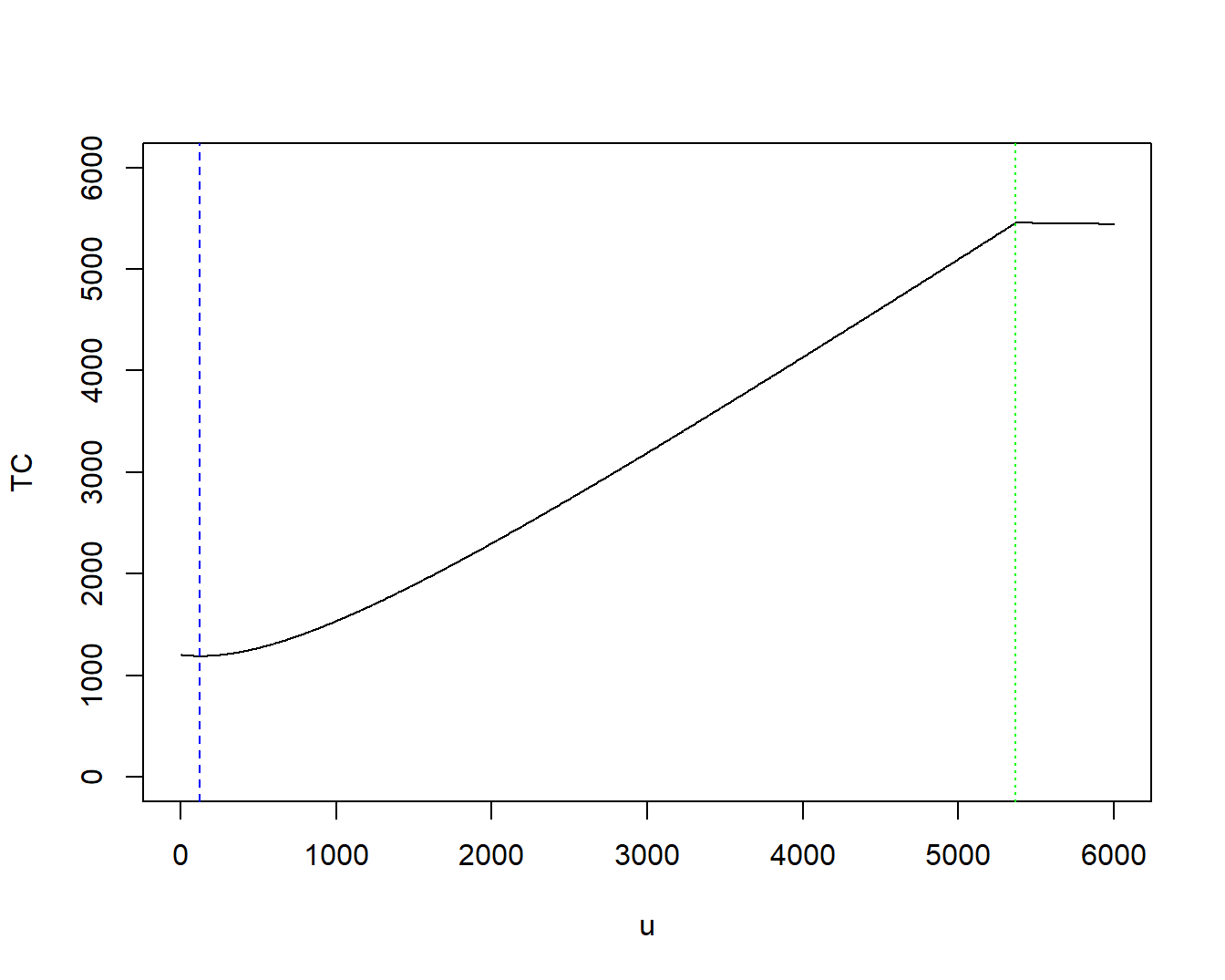
Figure 3.1: Total Cost using Value at Risk for an Upper Limit Policy. The blue vertical dashed line marks the point of optimal (lowest) cost. The green vertical dashed line marks that point where the upper limit equals the quantile of the confidence level, \(F_{0.98}^{-1}\).
There are several insights that we can get from this example.
- Suppose that in equation (3.1), one uses the \(ES\) measure instead of the \(VaR\). Then, by examining Table 2.2, one can see that the differential association with \(u\) remains unchanged and so the optimal upper limit remains unchanged. This is comforting to managers of risk. The optimal amount of risk retention does not matter when deciding between the value at risk and the expected shortfall.
- Suppose that a risk manager wishes to use the total cost procedure optimizing over the coinsurance parameter (keeping the deductible and upper limit fixed). Then referring to equation (3.2) and Table 2.2, one can see that this is problematic. That is, both the risk measure and the cost of ceding the risk are linear in this parameter so that a unique optimum does not exist.
- In the preceding example, the optimal upper limit (125.3171) seems low especially when compared to the mean risk (1,000 for this example). The result is more intuitively appealing if one considers optimizing over deductibles that, from equation (3.2) and Table 2.2, gives exactly the same result. That is, if the risk owner wants to outsource the small nuisance claims in a cost-efficient way, then a deductible makes sense and this procedure provides an intuitively plausible result.
Despite the limitations listed above, the total cost approach is attractive because it is simple and intuitively appealing. Now, suppose that we have available a menu of risk transfer options that depend on risk retention parameter \(\theta\). Each option has an associated cost \(RTC(\theta)\) that may be market driven from an external insurer or reinsurer. Then, the total cost is \(TC =\) \(RM[\theta] +\) \(RTC(\theta)\) that one could minimize by taking derivatives and solving for zero to get \[ \partial_{\theta} ~RM[\theta] = - \partial_{\theta} RTC(\theta) \Rightarrow \frac{\partial_{\theta} ~RM[\theta]}{- \partial_{\theta} ~RTC(\theta) } = 1 . \] This provides a necessary condition for achieving an optimal total cost. As described in Section 2.3.2, ratios of differentials are intuitively appealing. Moreover, as seen in this section, they also provide information as to when we are close to an optimal total cost.
3.2.2 Total Cost Optimal Designs
This section examines the theoretical literature on optimal design, building on the work of Cai and Chi (2020) in the realm of risk measures. To formalize the preceding discussion, the optimal design aims to minimize \(RM[T_g(X)]\) over a set of retention functions, with \(RM\) representing a given risk measure. This optimal design encompasses three key dimensions:
- A set of feasible retention functions.
- A premium principle for calculating \(RTC(g)\).
- A risk owner’s objective function \(RM\).
Initially proposed by Cai and Tan (2007), this approach determined the optimal choice of the retention parameter for an upper limit policy for a \(VaR\) risk measure (also done for the \(ES\) measure). Expanding on this work, the same team of authors in Cai et al. (2008) identified the upper limit policy as optimal when (1) the choice of feasible ceded loss, \(X-g(X)\), function is convex increasing, (2) the expected value principle is used for calculating risk transfers, and (3) the objective function is either the \(VaR\) or the \(ES\).
Cai and Chi (2020) further trace various contributions that propose alternative optimal functions as the set of retention/ceded loss functions varies. For different sets, with the \(VaR\) objective function, the optimal policy may be either upper limit, a one-layer policy of the form \(g(x) =\) \(x- \min[(x-a)_+,b-a)]\), or a truncated upper limit of the form \(g(x) =\) \(x - (x-d)_+I(x \le m)\), where \(a, b, d, m\) are constants. However, when using the \(ES\) risk measure as an objective function, it turned out that the choice of feasible functions was robust in the sense that the upper limit policy was optimal for these sets.
Instead of separately discussing the optimality under \(VaR\) and \(ES\) measures, the literature has subsequently cast both problems as special cases of a general distortion risk measure defined in Section 2.5.3. Not surprisingly, the optimal design is contingent upon the choice of the risk measure.
Constrained Optimization Strategy. As another extension, this literature has separated the total risk into two components, the uncertainty of retained risks and the risk transfer cost. Specifically, the objective is to identify contract types that minimize the uncertainty of the risk \(RM[g(X)]\) subject to the constraint \(RTC(g) \le\) \(RTC_{max}\) for a fixed maximal risk transfer cost, denoted here as \(RTC_{max}\). The solution to this optimization problem is that a piece-wise functional strategy is optimal. Examples of this approach can be found in the budget constrained work of Lo (2017) and Cheung, Chong, and Lo (2019).
This separation is intuitively plausible. One rationale is that the marketplace, and hence prices, for insurance/reinsurance costs differs from the capital requirements faced by the risk owner. The risk owner might achieve the desired protection below a specific “reservation” price, an aspect that is explicitly recognized in a budget constrained set-up. Another justification is the discrepancy between retained risks and risk transfer costs in the timing and accounting. Payments for risk transfer costs are typically known early on, sometimes being made at the beginning of a contract period. In contrast, many risks take years to develop before their full impact is discernible. This difference in timing may also warrant different accounting treatments. Hence, it might be limiting to aggregate these components into a total cost; a separate treatment is more intuitively appealing.
Starting from the following section, we delve into the constrained optimization approach. The work cited in this section primarily concentrates on establishing conditions to optimize the structure of the risk transfer agreement. In contrast, we assume the contract form as known and aim to select the most suitable parameters. An advantage of working with this “reduced” problem is that we are able to make contributions to the study of multivariate risks, a central theme of this book.
Video: Section Summary
3.3 Constrained Optimization
Risk managers seek to reduce the uncertainty of retained risks and minimize the costs of offloading risks. Our approach, consistent with modern asset portfolio analysis, is to treat this as an optimization problem. A general strategy that one might adopt consists of optimizing both quantities simultaneously, known as vector optimization, cf. Boyd and Vandenberghe (2004), Section 4.7. Due to the complexity of this strategy, we use the far more widely adopted approach and look to constrained optimization. In the context of this problem treated in this chapter, we seek to find those risk retention parameters in the vector \(\boldsymbol \theta\) that
\[\begin{equation} \begin{array}{ll} {\small \text{minimize}}_{\boldsymbol \theta} & ~~~~~RM[g(X;\boldsymbol \theta)] \\ {\small \text{subject to}} & ~~~~~RTC(\boldsymbol \theta) \le RTC_{max} ~~. \end{array} \tag{3.3} \end{equation}\]
We seek to minimize the uncertainty in retained risks summarized by \(RM[g(X;\boldsymbol \theta)]\) but are limited to the aptly termed “budget” constraint \(RTC(\boldsymbol \theta) \le RTC_{max}\). The collection of those values of \(\boldsymbol \theta\) that satisfy this constraint is known as the feasible set. Additional terminology is collected in Appendix Section 3.6.3.
Before further discussing this problem in the risk retention situation, we first provide further context by describing applications in closely related areas.
3.3.1 Applications in Other Fields
It is likely that many readers are familiar with constrained optimization from their studies of economics, finance, and data science. As a refresher, several well-known problems can be addressed using constrained optimization.
Economics. Numerous fundamental problems in microeconomics can be solved using constrained optimization. For instance, consider a scenario where a consumer selects the most preferred bundle from a budget set. The consumer has a utility function (\(U\)) defined over two goods, such as the quantity of milk (\(C_1\)) and butter (\(C_2\)). The objective is to maximize the utility of these goods, \(U(C_1, C_2)\), but is limited by a budget constraint of the form \(P_1 C_1 + P_2 C_2 \le Budget_0\). Here, \(P_1\) is the price of milk, \(P_2\) is the price of butter, and \(Budget_0\) is the maximum amount that the consumer has to spend on these goods.
Another typical microeconomics problem likely familiar to many readers is a cost minimization problem. For example, a firm produces output using amounts of capital \(Cap\) and labor \(Labor\) according to a Cobb-Douglas production function of the form \(f(Cap,Labor) = A_3 Cap^{a_1} Labor^{a_2}\). The firm must produce at least \(Product_0\) of output. Subject to this constraint, the firm seeks to choose inputs \(Cap\) and \(Labor\) to minimize costs given by \(Cost(r,w) = rCap +wLabor\), where \(r\) is a rental rate for capital and \(w\) is a wage rate.
Finance. Perhaps the example most well-known to risk managers is the asset allocation problem. Markowitz (1952) proposed a theory to construct a portfolio of assets in order to maximize expected returns with a given level of uncertainty. Because of the relevance of asset allocations to our interests, Section 3.4 provides a detailed introduction to this problem.
Data Science. Optimization is heavily utilized in data science, statistics, and machine learning. Many, if not almost all, methods developed for fitting and prediction can be viewed as some form of optimization. Constrained optimization problems appear frequently, particularly in those methods that seek to develop a balance between the ability to fit a model to data and a desire to reduce model complexity. To illustrate, both lasso and ridge regressions can be viewed as constrained problems that balance fit and complexity (see, for example, Exercise 3.1). Another data science example of constrained optimization is support vector machines, a classification method (see, for example, Hastie, Tibshirani, and Friedman (2009)).
3.3.2 An Upper Limit Contract
To demonstrate how the constrained optimization approach works within the realm of risk retention, we initially consider an upper limit contract. In this scenario, only a single parameter varies, making optimization relatively straightforward. This section provides specific details to establish a foundation for tackling more complex settings. We consider only the value at risk measure here but describe other risk measures in the following Section 3.5.
One aspect that simplifies the problem is that the constraint function \(RTC(u)\) can be assumed to be monotonic decreasing in the choice variable \(u\). Consequently, as we increase retention by increasing \(u\), the risk transfer cost stays the same or becomes smaller. For instance, in the baseline scenario with no additional surcharges, \(RTC(u)\) represents only the expected transferred risk. With the risk retention function from equation (2.6), considering only an upper limit means no coinsuring of risks (\(c=1\)) and no deductible (\(d=0\)). Thus, with equation (2.7), we have \[\begin{equation} RTC(u) = \mathrm{E}(X) - \mathrm{E}(X \wedge u) = \int_u^{\infty} ~ [1-F(z)] ~dz, \tag{3.4} \end{equation}\] that can readily be seen to be monotonic decreasing in \(u\). Define \(u_{max}\) to be the smallest value of \(u\) that satisfies the constraint in Display (3.3). Thus, the feasible interval over which we seek to minimize the uncertainty of retained risks is \([u_{max}, \infty)\). Note that we could also use the notation \(u_{max}(RTC_{max})\) to remind ourselves that the value of \(u_{max}\) depends on the choice of \(RTC_{max}\).
For the uncertainty measure, consider the value at risk. From equation (2.10) , we see that the value at risk is \(VaR_{\alpha}(X \wedge u) = \min(F^{-1}_{\alpha}, u)\) – see the right panel of Figure 3.2. Thus, the problem is to \[\begin{equation} \boxed{ \begin{array}{lc} {\small \text{minimize}}_u & \min(F^{-1}_{\alpha}, u) \\ {\small \text{subject to}} & u \ge u_{max} . \end{array} } \tag{3.5} \end{equation}\] As evident from Figure 3.2, like the constraint function, the uncertainty measure is also monotonic in \(u\), but is monotonic increasing, not monotonic decreasing. Thus, we minimize the objective function by making the decision variable \(u\) as small as possible. Formally, by changing the value of \(RTC_{max}\), we can think about two cases.
- In the first case, suppose that \(F^{-1}_{\alpha} \ge u_{max}\). In this case, the smallest that the upper limit \(u\) can be and still lie within the feasible region is \(u^* = u_{max}\) with this as the value at risk.
- In the second case, suppose that \(F^{-1}_{\alpha} < u_{max}\). In this case, for any upper limit \(u\) in the feasible region, \(u \ge u_{max}\) (\(> F^{-1}_{\alpha}\)), has the minimal value at risk \(F^{-1}_{\alpha}\).
Summarizing, the optimal value at risk is \[\begin{equation} VaR_{\alpha}(X \wedge u)^* =VaR_{\alpha}(X \wedge u_{max}) = \left\{ \begin{array}{cc} u_{max} & \text{if} \ u_{max} \le F^{-1}_{\alpha} \\ F^{-1}_{\alpha} & \text{if} \ u_{max} > F^{-1}_{\alpha} \\ \end{array} \right. ~~. \tag{3.6} \end{equation}\]
Example 3.2. Optimal Upper Limits Using a Pareto Distribution. Continuing with the example from Section 3.2.1, we use a Pareto distribution but with parameters \(\eta = 3\) and \(\gamma = 1000\). We also assume a confidence level \(\alpha = 0.90\). For this distribution and confidence level, the quantile is \(F_{0.90}^{-1} = 1154.435\). The risk transfer cost without loading is given in equation (3.4).
Results are in Figure 3.2. The left-panel shows the maximum upper limit \(u_{max}\) as a function of the maximal risk transfer \(RTC_{max}\). The right-hand panel shows the optimal value at risk, from equation (3.6), as a function of the maximal risk transfer. Note that the value at risk is bounded from above by \(F_{0.90}^{-1}\); all maximal risk transfers below this point produce the same value at risk.
R Code for Example 3.2
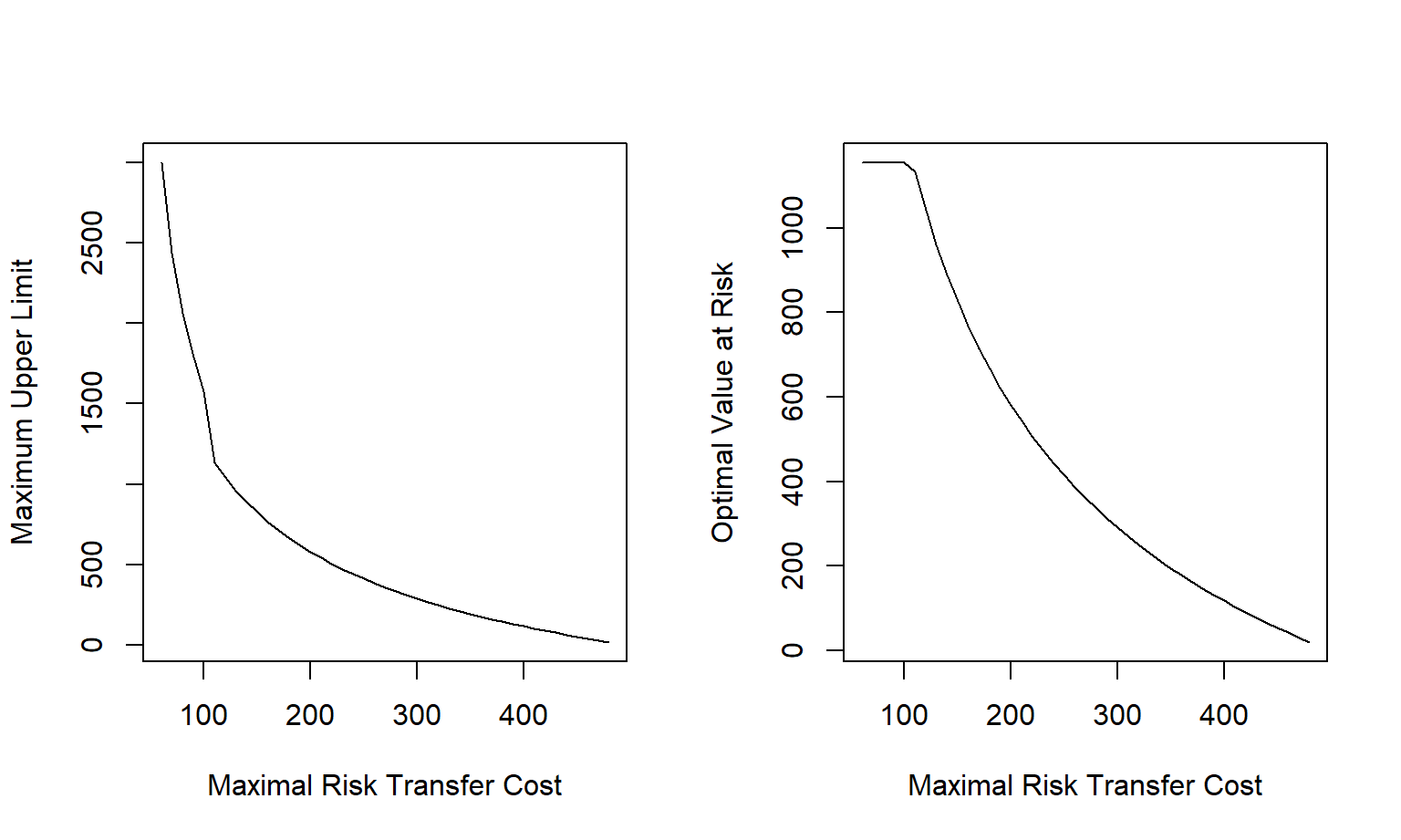
Figure 3.2: Maximum Upper Limit and Optimal Value at Risk versus Required Maximal Risk Transfer Cost
3.3.3 The Lagrangian
With constrained optimization problems, one can often employ the Lagrange method for optimization. This is a classical approach for minimizing (or maximizing) a function subject to equality constraints. To illustrate, for the risk retention problem in Display (3.3), suppose that we are only interested in risk retention parameters that achieve the maximal risk transfer cost, that is, those values of \(\boldsymbol \theta\) so that \(RTC(\boldsymbol \theta) = RTC_{max}\). Then, the corresponding Lagrangian is
\[\begin{equation} LA(\boldsymbol \theta, LM) = RM[g(X;\boldsymbol \theta)] + LM \left\{RTC(\boldsymbol \theta) - RTC_{max} \right\} . \tag{3.7} \end{equation}\]
In this classical approach, one determines the parameters in \(\boldsymbol \theta\) and the new parameter \(LM\) that optimize the function \(LA\). Thus, the Lagrange method essentially turns a constrained problem into an unconstrained problem.
The constraint is said to be active or binding when, at the optimum \(\boldsymbol \theta^*\), we have \(RTC(\boldsymbol \theta^*) = RTC_{max}\). In many of our problems (but not all), this is a natural consequence of the constraints on the risk transfer cost. If the constraint is binding then we can treat the problem as an equality constrained problem.
To interpret the new parameter \(LM\), we can take derivatives. Specifically, we can take a derivative of the Lagrangian with respect to the \(i\)th variable in \(\boldsymbol \theta\). If we evaluate it at the optimum, then this derivative equals zero. Thus, we see that the Lagrange multiplier can be expressed as
\[\begin{equation} LM = -\frac{\partial_{\theta_i} ~RM[g(X;\boldsymbol \theta)]}{\partial_{\theta_i} ~RTC(\boldsymbol \theta)} = RM^2_i \tag{3.8} \end{equation}\]
at the optimal value of \(\boldsymbol \theta\). This ratio of the differential change is the uncertainty of retained risks per unit differential change in the risk transfer cost, similar to that described in Section 2.3.2. In earlier work, Frees (2017) called this the risk measure relative marginal change, or \(RM^2\) change, an intuitively appealing measure. We saw how to compute these quantities in Section 2.3.2.
In constrained optimization problems, it can be helpful to check that both the objective function (\(RM[g(X;\boldsymbol\theta)]\)) and the constraint function (\(RTC(\boldsymbol\theta)\)) are convex (in \(\boldsymbol\theta\)). If so, then any local optimal point will be a global optimal point. However, as we saw in Section 2.4, the risk retention problem in Display (3.3) is not a convex optimization problem in general. This means that the local optimum that we calculate is not guaranteed to be a global optimum point, implying that the analyst must take care in interpreting results.
3.3.4 A General Constrained Optimization Problem
Most of the risk retention problems considered in this text can be written as a special case of the following optimization problem:
\[\begin{equation} \begin{array}{lcc} {\small \text{minimize}}_{\bf z} & f_0(\bf z) & \\ {\small \text{subject to}} & f_{con,j}({\bf z}) \le 0 & j \in CON_{in} \\ & f_{con,j}({\bf z}) = 0 & j \in CON_{eq} . \end{array} \tag{3.9} \end{equation}\]
In this display, the objective \(f_0(\cdot)\) and the constraint functions \(f_{con,j}(\cdot)\) all depend on the decision variables \({\bf z}=(z_1, \ldots, z_{p_z})^{\prime}\). Some of the constraints are of the inequality type and those are members of the set \(CON_{in}\). In the same way, equality constraints are members of the set \(CON_{eq}\). Often, the decision variables are simply the risk retention parameters so \({\bf z} = \boldsymbol \theta\). However, in some cases we let one or more retention variables be fixed in advance and so they are not decision variables. In addition, for some risk measures we will include additional auxiliary variables as elements of \({\bf z}\) in the optimization that are not risk retention parameters. So, we allow decision variables and risk retention parameters to differ with differing notation; we employ a \(p\) dimensional vector of risk retention variables and a \(p_z\) dimensional vector of decision variables.
Generally, \(f_0\) is a risk measure that we wish to minimize subject to constraints on the risk transfer costs. For some problems, \(f_0\) can be a risk transfer cost that we wish to minimize subject to constraints on a maximum acceptable level of risk determined by the risk measure.
An equivalent problem formulation that is mathematically more elegant can be written as \[ \boxed{ \begin{array}{lcc} {\small \text{minimize}}_{{\bf z}} & f_0({\bf z}) & \\ {\small \text{subject to}} & f_{con,j}({\bf z}) \le 0 & \text{for all } j .\\ \end{array} } \] Display (3.9) reduces to the simpler formulation simply by dropping the equality constraints. However, one can also go the other direction. Starting with the simpler form, if we use two inequality constraints of the form \(f_{con,j}({\bf z}) \le 0\) and \(-f_{con,j}({\bf z}) \le 0\), this is equivalent to an equality constraint.
We work with the seemingly more cumbersome formulation in Display (3.9) because this form is used in many software presentations - it is common for algorithms to separate considerations for equality constraints from those of inequality constraints. Another form, used in many economic applications, involves separating parameter constraints and assuming parameters are non-negative; this aids in interpreting results. For example, in later chapters we will work with multivariate risks and, in some of those applications, \(\theta_i=0\) may mean the full risk transfer of the \(i\)th risk, something that is of special importance for risk retention problems. This convention could also easily be adopted, see Section 11.3.1.
In many instances, we are able to solve a constrained optimization problem numerically by relying on software. Nonetheless, to gain insights into how the software works and sometimes reformulate problems into ones that are numerically more stable, it is helpful to think about the underlying theory.
The classical approach using Lagrangians for optimization subject to equality constraints can be extended to include inequality constraints. For Display (3.9), the associated Lagrangian is
\[\begin{equation} LA\left({\bf z},\mathbf{LMI},\mathbf{LME}\right) = f_0({\bf z}) + \sum_{j \in CON_{in}} LMI_j ~f_{con,j}({\bf z}) + \sum_{j \in CON_{eq}} LME_j ~f_{con,j}({\bf z}) , \tag{3.10} \end{equation}\]
where \(\mathbf{LMI} = \left(LMI_1, \ldots, LMI_{m_{in}} \right)^{\prime}\) and \(\mathbf{LME} = \left(LME_1, \ldots, LME_{m_{eq}} \right)^{\prime}\) are Lagrange multiplier vectors for the inequality and equality constraints, respectively.
Video: Section Summary
3.4 Asset Allocation Problem
Asset allocations can be readily seen as a type of constrained optimization problem.
3.4.1 Markowitz Portfolio Optimization
To describe how portfolios are formed, we first introduce a bit of notation. An investor considers:
- \(p\) asset risks \(\mathbf{R} =(R_1, \ldots, R_p)^{\prime}\), each with mean \(\mathrm{E }(R_j)\) and variance \(\mathrm{Var }(R_j) = \Sigma_{jj}\), \(j=1, \ldots,p\).
- The dependence of a pair of risks is measured by a covariance \(\mathrm{Cov}(R_i, R_j) = \Sigma_{ij}\). The \(p \times p\) matrix \(\boldsymbol \Sigma\) collects variances and covariances (with \(\Sigma_{ij}\) as the element in the \(i\)th row and \(j\)th column).
- Let \(c_j\) be the fraction of an investor’s wealth in the \(j\)th asset and \(\mathbf{c} =(c_1, \ldots, c_p)^{\prime}\) is the vector of investment allocations. These are the choices that the investor makes and are the decision variables for this problem.
- The weighted sum \(\sum_{j=1}^p c_j R_j = \mathbf{c}^{\prime}\mathbf{R}\) gives the investor’s portfolio return.
- For a given allocation vector \(\bf c\), the portfolio mean is \(\mathrm{E }[\mathbf{c}^{\prime}\mathbf{R}] = \mathbf{c}^{\prime} ~\mathrm{E}(\mathbf{R})\) and the variance is \(\mathrm{Var}[\mathbf{c}^{\prime}\mathbf{R}] = \mathbf{c}^{\prime} ~\boldsymbol \Sigma~\mathbf{c}\).
Asset Allocation Problem. The asset allocation problem can be expressed as one of three following forms: \[\begin{equation} \boxed{ \begin{array}{lc} {\small \text{maximize}}_{\mathbf{c}} & \mathbf{c}^{\prime} ~\mathrm{E}(\mathbf{R}) \\ {\small \text{subject to}} & \mathbf{c}^{\prime} ~\boldsymbol \Sigma~\mathbf{c} \le Var_0 \\ \end{array} } \tag{3.11} \end{equation}\] \[\begin{equation} \boxed{ {\small \text{maximize}}_{\mathbf{c}} \ \ \ \mathbf{c}^{\prime} ~\mathrm{E}(\mathbf{R}) - \lambda_{Port} ~\mathbf{c}^{\prime} ~\boldsymbol \Sigma~\mathbf{c} } \tag{3.12} \end{equation}\] \[\begin{equation} \boxed{ \begin{array}{lc} {\small \text{minimize}}_{\mathbf{c}} & \mathbf{c}^{\prime} ~\boldsymbol \Sigma~\mathbf{c} \\ {\small \text{subject to}} & \mathbf{c}^{\prime} ~\mathrm{E}(\mathbf{R}) \ge Req_0 \\ \end{array} } \tag{3.13} \end{equation}\] Here, \(Var_0\) is the maximal portfolio variance, \(\lambda_{Port}\) is a penalty parameter that controls the trade-off between the portfolio mean and variance, and \(Req_0\) is the required expected portfolio return. Displays (3.11)-(3.13) are equivalent in the sense that they trace the same frontier by varying the values of \(Var_0\), \(\lambda_{Port}\), and \(Req_0\).
Example 3.3. Portfolio of Insurance Stock Returns. This is a continuation of Example 1.1. The portfolio frontier is displayed in Figure 3.3 for these data. In addition to the frontier, stocks with the highest mean and lowest standard deviation are displayed for comparison purposes. Also shown is the equally weighted portfolio, where \(c_j = \frac{1}{8}\) for each \(j\).
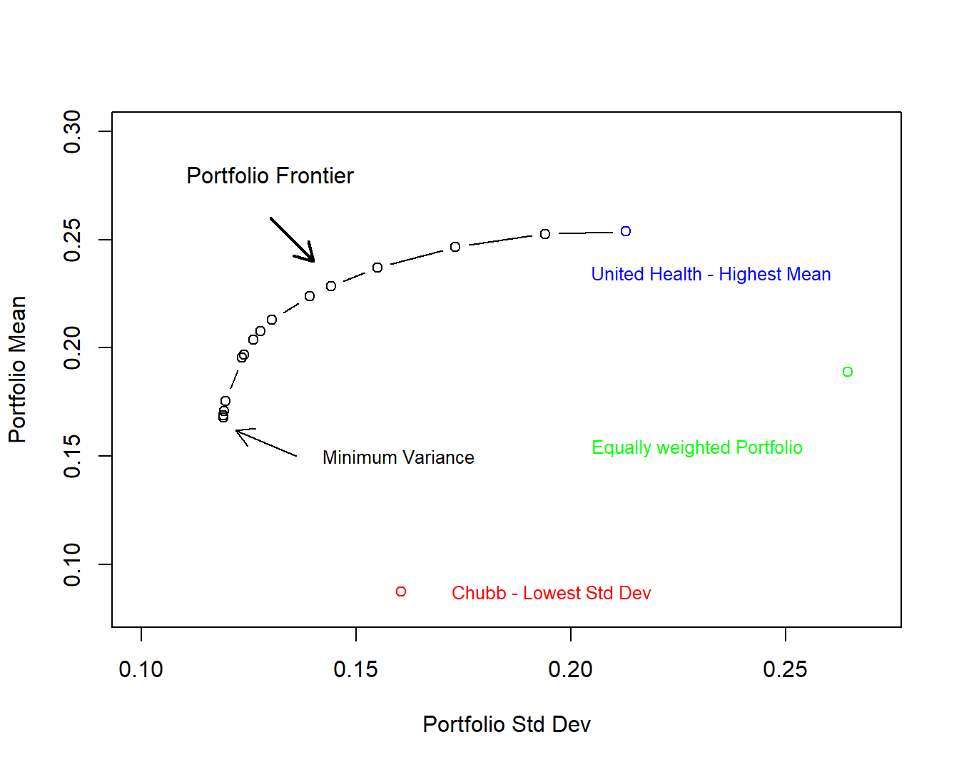
Figure 3.3: Frontier of Portfolio Standard Deviations and Means
R Code for Example 3.3
Three portfolios were created, all subject to the constraint that the allocation choices sum to one, \(\sum_j c_j =\mathbf{c}^{\prime}\mathbf{1} = 1\) (the bold-faced \(\mathbf{1}\) is a vector of ones). One is the equally weighted portfolio, the second a “Markowitz” portfolio (taking \(\lambda_{Port}=5\)), and the third is a “minimum variance” portfolio. You can think of the third as a special case of the Markowitz portfolio in Display (3.13) where the minimal expected return \(Req_0\) is so small that it can be neglected. The three sets of portfolio weights are shown in Figure 3.4. The Markowitz portfolios were calculated using the R package CVXR - you can learn more about this package at the website https://cvxr.rbind.io.
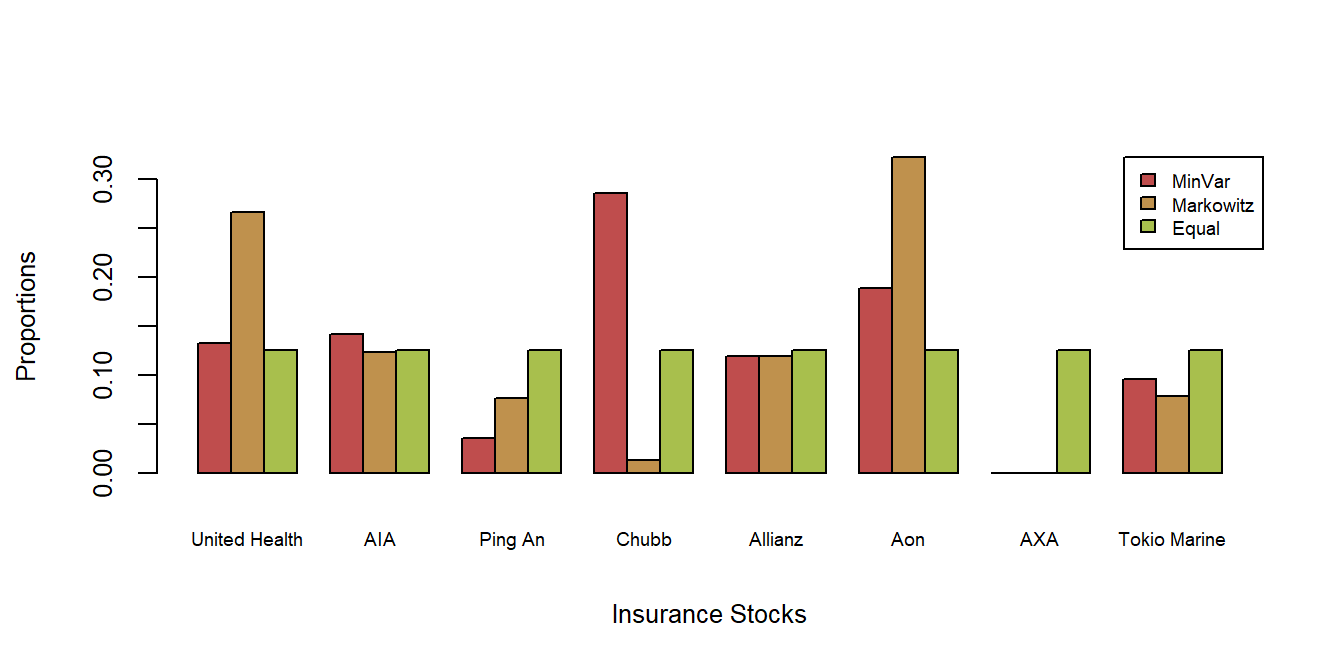
Figure 3.4: Three Sets of Portfolio Allocations, by Insurer
The first three columns of Table 3.1 summarize the performance of the portfolios on the training sample as measured by the annual return, standard deviation, and the Sharpe ratio. Many financial analysts use the Sharpe ratio, the mean minus a risk-free rate divided by the standard deviation, to summarize portfolio performance. As anticipated, the MinVar minimum variance portfolio had the lowest standard deviation. With a zero risk-free rate, the Markowitz portfolio is the strongest performer for the training sample based on the Sharpe ratio.
Columns four through six of Table 3.1 summarize the performance of the portfolios on the test sample. Interestingly, the MinVar portfolio had a high test standard deviation (nearly the same as the two other portfolios). Based on the Sharpe ratio criterion, it was also the strongest performer.
| Train Ann Return | Train Std Dev | Train Sharpe (Rf=0) | Test Ann Return | Test Std Dev | Test Sharpe (Rf=0) | |
|---|---|---|---|---|---|---|
| MinVar | 0.164 | 0.119 | 1.378 | 0.168 | 0.143 | 1.178 |
| Markowitz | 0.203 | 0.126 | 1.614 | 0.166 | 0.143 | 1.160 |
| Equal | 0.173 | 0.130 | 1.329 | 0.155 | 0.142 | 1.093 |
To get a better sense of the portfolios’ performance on the test sample, Figure 3.5 shows cumulative returns. All three are close to one another.
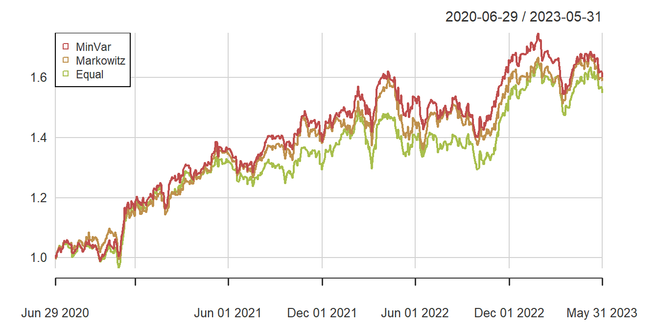
Figure 3.5: Cumulative Portfolio Returns (Test Sample)
One cannot conclude too much from these results. Practicing analysts will use this approach while conducting more extensive testing by varying the training period, the test period, and the sample of stocks (risks) selected. Readers are invited to experiment with the code to determine their own optimal portfolios, see, for example Exercise 3.3.
3.4.2 Constraining Markowitz Portfolio Optimization
The popularity of the Markowitz portfolio approach is due in part to the fact that there is a simple closed form solution to the problem (see Exercises 4.2 and 4.3).
Moreover, given knowledge of the means, variances, and covariances, the optimization problem summarized in Displays (3.11)-(3.13) is typically convex (assuming a semi-positive definite covariance matrix). As will be discussed in Chapter 4, this means that fast solvers are readily available for the problem. Convexity will also mean that one can impose additional linear (or convex) constraints on the problem and still achieve quick, reliable solutions. Display (3.14) exhibits several additional constraints regularly employed by practicing analysts: \[\begin{equation} \boxed{ \begin{array}{cl} \mathbf{c}' {\bf 1}= 1 & \text{full investment constraint} \\ \hline c_j \ge 0, c_j \le 1 & \text{short/long constraints} \\ \mathbf{c}' {\bf 1}= 0 & \text{dollar-neutral constraint}\\ lower_j \le c_{j} \le upper_j & \text{holding constraint} \\ \hline \sum_j |c_j| \le Bound_{leverage} & \text{leverage constraint} \\ \sum_j |c_j - c_{0,j}| \le Bound_{turnover} & \text{turnover constraint }\\ & \ \ c_{0,j} \text{ represents the} \\ & \ \ \ \ \ \ \text{current position} \\ \end{array} . } \tag{3.14} \end{equation}\] The first condition, “full investment constraint,” ensures that one can interpret the allocations \(c_j\) as fractions of a given wealth amount invested in a portfolio. The second condition excludes “short selling” as is common in financial investment transactions; an investor may not take a negative position on a risk. The other conditions place limits on the portfolio allocations to meet differing investment strategies.
Video: Section Summary
3.5 Constrained Optimization Approach to Risk Retention
To cultivate an understanding of how the constrained optimization approach applies to risk retention problems, let us examine several special cases of the risk retention function (2.6). Working with a single risk and a limited number of risk retention parameters enables us to obtain precise analytical results in many instances, aiding in the development of intuition for the process.
3.5.1 Upper Limits and ES
I now extend the discussion of upper limit contracts begun in Section 3.3.2 to include another uncertainty measure, the expected shortfall. From equation (2.11), the expected shortfall is \[ \begin{array}{ll} ES_{\alpha}(X \wedge u) &= \left\{ \begin{array}{cc} u & \text{if} \ u \le F^{-1}_{\alpha} \\ F^{-1}_{\alpha} + \frac{1}{1-\alpha} \left\{E [X \wedge u] - E [X \wedge F^{-1}_{\alpha}]\right\} & \text{if} \ u > F^{-1}_{\alpha} \\ \end{array} \right. . \end{array} \] Thus, the problem is \[\begin{equation} \boxed{ \begin{array}{lc} {\small \text{minimize}}_u & ES_{\alpha}(X \wedge u) \\ {\small \text{subject to}} & u \ge u_{max} , \end{array} } \tag{3.15} \end{equation}\] where we can use the same maximum upper limit \(u_{max}\) for a given maximal risk transfer \(RTC_{max}\) as in the value at risk case discussed in Section 3.3.2. Unlike the value at risk case, the objective function is strictly increasing in \(u\) (assuming continuity of the distribution function). The smallest that the upper limit \(u\) can be and still be within the feasible region is \(u^* = u_{max}\). Thus, this represents the optimal choice of \(u\) with the expected shortfall evaluated at \(u^*\). We summarize the optimal objective function as \[\begin{equation} {\small \begin{array}{ll} &ES_{\alpha}(X \wedge u)^* =ES_{\alpha}(X \wedge u_{max}) \\ & \ \ \ = \left\{ \begin{array}{cc} u_{max} & \text{if} \ u_{max} \le F^{-1}_{\alpha} \\ F^{-1}_{\alpha} + \frac{1}{1-\alpha} \left\{E [X \wedge u_{max}] - E [X \wedge F^{-1}_{\alpha}]\right\} & \text{if} \ u_{max} > F^{-1}_{\alpha} \\ \end{array} \right. . \end{array} \tag{3.16} } \end{equation}\]
Example 3.4. Optimal Upper Limits with \(ES\) Using a Pareto Distribution. This is a continuation of Example 3.2. Because the risk transfer cost is the same, we can refer to the left-hand panel of Figure 3.2 to see the maximum upper limit \(u_{max}\) as a function of the maximal risk transfer \(RTC_{max}\). The relationship between the maximal risk transfer \(RTC_{max}\) and the optimal expected shortfall \(ES_{\alpha}(X \wedge u)^*\) is summarized in Figure 3.6. In this figure, a horizontal green dashed line is given at \(F_{0.90}^{-1} = 1,154.43\) where this is a break in the expression for \(ES_{\alpha}(X \wedge u)^*\). One can see that this is smooth, at least compared to the similar graph for the value at risk in the right-hand panel of Figure 3.2.
R Code for this Figure
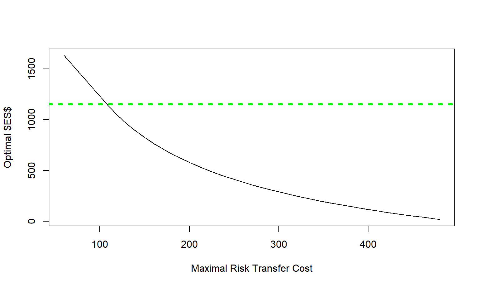
Figure 3.6: Optimal Upper Limit and \(ES\) versus Maximal Risk Transfer Cost
Comparing Value at Risk to Expected Shortfall
From the discussions in Sections 3.3.2 and 3.5.1 and a comparison of equations (3.6) and (3.16), one sees that the optimal upper limit in both cases is \(u_{max}\) when \(u_{max} \le F^{-1}_{\alpha}\). This is emphasized in the Figure 3.7 comparison.
R Code for the Figures
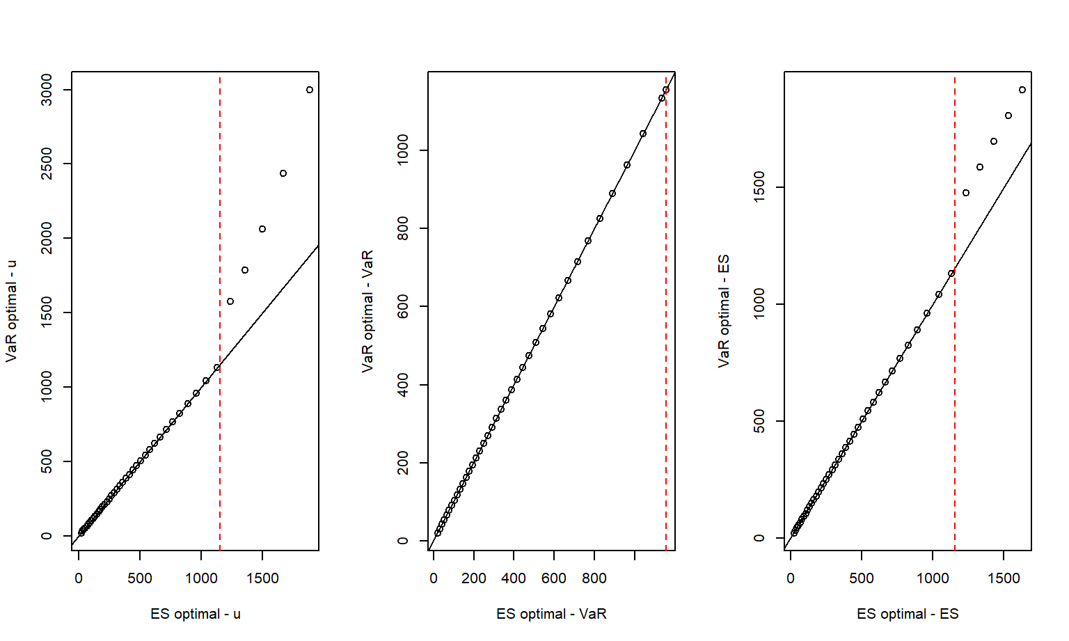
Figure 3.7: Comparing Retentions and Summary Measures from VaR and ES Optimization. The vertical dashed red line marks the alpha percentile of the distribution function.
In Exercise 3.2, readers are asked to show that the range value at risk measure \(RVaR_{(\alpha,\beta)}(X \wedge u)\) is monotone increasing in \(u\). This result is not surprising given that this risk measure captures the value at risk and the expected shortfall as special cases. One can use this fact to readily use this general risk measure to determine an optimal parameter value for the upper limit case considered in this section.
3.5.2 Other Coverages
This section summarizes some interesting consequences of constrained optimization for other coverages using first principles. Later, in Chapter 11, I show how to obtain similar results using the Karush-Kuhn-Tucker, or KKT, conditions that hold for general constrained optimization problems.
Upper Limits with Coinsurance
Now consider a contract with an upper limit \(u\) and coinsurance \(c\) but assume there is no deductible so \(d=0\). Starting with the value at risk, from equation (2.10) with \(d=0\), one has \[ VaR_{\alpha}\{g[X;\boldsymbol \theta =(d=0, c, u)]\} = c \left[F^{-1}_{\alpha} \wedge u \right] . \] For the risk transfer cost, let us write \[ \begin{array}{ll} RTC(c,u) & = \mathrm{E}[X - c(X \wedge u)] = \mathrm{E}(X) - c\int_0^u ~ [1-F(z)] ~dz \\ & = \mathrm{E}(X) - cH(u) . \end{array} \] Here, \(H(\cdot)\) is the integral of the survival function, \(1-F(\cdot)\).
To determine values of \(c\) and \(u\) that minimize \(VaR_{\alpha}[g(X)]\) subject to the constraint \(RTC(c,u) \le RTC_{max}\), one strategy is to fix the value of \(c\), solve the constraint problem, and then use that value of \(c\) that produces the smallest value at risk. To simplify the presentation, assume that \(RTC_{max}\) is sufficiently small so that the constraint is binding. Now, by equating the risk transfer cost to its maximum value, one can write the maximum upper limit in terms of the maximum cost and the coinsurance parameter as \[ \begin{array}{rl} RTC(c,u_{max}) = RTC_{max} \Rightarrow & \mathrm{E}(X) - cH(u_{max}) = RTC_{max} \\ \Rightarrow & u_{max}(c) =u_{max} = H^{-1}\left(\frac{\mathrm{E}(X) - RTC_{max}}{c}\right) .\\ \end{array} \] Similar to equation (3.6), the solution to this subproblem is \[ VaR_{\alpha}(X \wedge u)_{opt,c} = F^{-1}_{\alpha} \wedge u_{max}(c). \] This solution is interesting. To begin, for very small values of \(c\), one sees that the value at risk is simply the quantile \(F^{-1}_{\alpha}\). To make \(u_{max}(c)\) as small as possible, make \(c\) as large as possible which is 1. Thus, the solution to the two parameter problem is the same as the one parameter problem described in Section 3.3.2 with \(c=1\).
Deductibles Only
From the definition of a deductible contract in Section 2.2.1, the risk owner is responsible for \[ g(X; d, c=1, u= \infty) = \left\{ \begin{array}{cc} 0 & \text{if} \ X < d \\ X-d & \text{if} \ X \ge d \\ \end{array} \right. = (X-d)_+ . \] That is, the risk owner has responsibility only for losses in excess of \(d\). As written above, this can be denoted using the subscript with a plus symbol ‘\((\cdot)_+\)’ meaning to take the positive part.
This can also be expressed as an upper limit as seen by the last equality. From this, we see that the deductible for the risk owner can be viewed as upper limit contract for the “risk taker.” The reverse is easier to interpret; an upper limit policy for the risk owner can be interpreted as a deductible policy for the entity that takes on the risk.
Deductible policies can easily be seen to be the mirror image of upper limit policies. That is, as the risk transfer cost is monotone decreasing in \(d\) and the risk measures \(VaR\), \(ES\), and \(RVaR\) are also monotone decreasing in \(d\). Hence, the constrained optimization techniques developed for upper limit policies work equally well with deductible policies. Our treatment focuses on upper limit policies as these are more useful when the risk owner is a firm.
Deductibles and Upper Limits
Introducing a deductible and an upper limit at the same time would be unusual if the risk owner is a firm but is common for risk owners that are insurers or, as will be discussed in Chapter 6, reinsurers. So, we now consider the case where the risk owner has no responsibility for small losses (less than \(d\)) and transfers excess large losses (losses in excess of \(u\)). For the objective function, let us now focus on the \(ES\). Although more complex, this function is smoother than the \(VaR\) measure and so may be easier to analyze.
The risk transfer cost from an expected value principle (without safety loadings) is \[ \begin{array}{ll} RTC(d,u) & = \mathrm{E}(X) - \left\{\mathrm{E} (X \wedge u) - \mathrm{E} (X \wedge d) \right\}. \end{array} \] The feasible region consists of those values of \((d,u)\) that satisfy \(RTC(d,u) \le RTC_{max}\). From the expression for \(RTC(d,u)\), we see that as \(RTC_{max}\) becomes large and approaches \(\mathrm{E}(X)\), the upper limit \(u\) becomes close to the lower limit \(d\), although there is no restriction on the value of \(d\). Conversely, as \(RTC_{max}\) becomes small and approaches 0, then \(d\) approaches 0 and \(u\) approaches \(\infty\).
Further, for the transfer to be feasible, we must have \(RTC(d,\infty) \le RTC_{max}\). That is, even if the risk owner retains all large losses, small losses must also be limited and so \(d\) must not be too large. For the largest possible value of the lower limit, define \(d_{max}\) to be the solution of the equation \(RTC(d,\infty) = RTC_{max}\). So, deductibles \(d^* \le d_{max}\) are in this feasible region. Now, we know that \(ES(d,u)\) is non-decreasing in \(u\) (see, for example, Table 2.2), so we want to choose \(u\) to be as small as possible. So, define \(u^* = u^*(d^*)\) to be the solution of the equation \(RTC(d^*,u)=RTC_{max}\).
How does the value of \(u^*\) depend on \(d^*\)? Differentiating this equation yields \[ \begin{array}{ll} 0 = \partial_{d^*} RTC(d^*,u^*) &= \left. \partial_{d} RTC(d,u) \right|_{d=d^*,u=u^*} \\ & \ \ \ \ \ \ \ + \left. \partial_{u} RTC(d,u) \right|_{d=d^*,u=u^*} \times \partial_{d^*} u^* \\ &= \left. \partial_{d} \mathrm{E} (X \wedge d) \right|_{d=d^*} - \left. \partial_{u} \mathrm{E} (X \wedge u) \right|_{u=u^*} \times \partial_{d^*} u^* \\ &= [1-F(d^*)] - [1-F(u^*)] \times \partial_{d^*} u^* \\ \Rightarrow & \partial_{d^*} u^* = \frac{1-F(d^*)}{1-F(u^*)} . \end{array} \] From this expression, we see that \(\partial_{d^*} u^* \ge 0\), so \(u^*\) decreases as \(d^*\) decreases.
Figure 3.8 visualizes these relationships. The upper left-hand panel shows the value of upper limits that achieve the max cost \(RTC_{max}\) for a given deductible. As determined theoretically, the slope is non-negative. The upper right-hand panel shows the corresponding \(ES\) where we see that the \(ES\) is increasing in \(d\).
It can be shown that \(RTC(d^*,u^*)\) is nondecreasing in \(d^*\) (see the online demonstration noted below). This means that the minimizing \(ES\) can be achieved by choosing \(d^* = 0\). For this value of \(d^*\), the optimal upper limit \(u.opt\) is the solution of the equation \(RTC(0,u)=RTC_{max}\). The lower left-hand panel of Figure 3.8 gives this upper limit as a function of the maximal risk transfer cost and the lower right-hand panel gives the corresponding value of the \(ES\). From this panel, we see that as the maximal risk transfer cost increases the uncertainty of retained risks as measured by \(ES\) decreases, as anticipated.
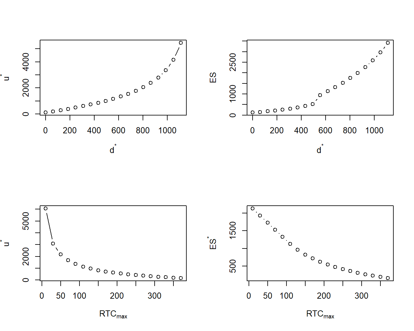
Figure 3.8: Deductible and Upper Limit Policy.
\(Under~the~Hood.\) Show the Derivative of the Optimal \(ES\)
Video: Section Summary
3.6 Supplemental Materials
3.6.1 Further Resources and Readings
Readers wanting a quick refresher to some basic statistical and actuarial concepts may refer to the online book, Actuarial Community (2020). In particular, Chapter 3 describes calculation of risk transfers for policies with coverage modifications, Chapter 10 provides an introduction to risk measures, and Chapter 18 summarizes limited expected value calculations.
The constrained optimization approach has long been known in the actuarial academic literature. See early contributions of Bühlmann (1970) and Daykin, Pentikäinen, and Pesonen (1994). The work of Bühlmann (1970) (page 114) traces its origins in the actuarial literature to contributions by Vajda (1962) and De Finetti (1940). See Frees (2017) and Lee (2017) for earlier investigations of the constrained optimization approach to risk retention most related to the approach in this book.
The supplemental Sections 3.6.4 and 3.6.5 provide additional descriptions of the best insurance designs from the economics and optimal reinsurance literatures.
3.6.2 Exercises
Exercise 3.1. Ridge and Lasso Regressions. As is customary in regression problems, assume that we have \(p+1\) variables from a sample of size \(n\). Denote observation \(i\) as \((x_{i1}, \ldots, x_{ip}, y_i) =\) \(({\bf x}_i, y_i)\) and think of \(y_i\) as a “response” variable to be explained or predicted by \(x_{i1}, \ldots, x_{ip}\). The traditional ridge and lasso regression estimators can be computed as the solution of \[ {\small \boxed{ \begin{array}{lc} {\small \text{minimize}}_{\boldsymbol \beta} & \frac{1}{n} \sum_{i=1}^n (y_i - {\bf x}_i^{\prime} \boldsymbol \beta)^2 \\ {\small \text{subject to}} & \sum_{j=1}^p |\beta_j |^s \le c_{regression} , \end{array} } } \] where \(s=2\) is for ridge regression and \(s=1\) is for lasso regression. Here, \(c_{regression}\) is a constant that limits the size of the regression coefficients \(\beta_1, \ldots, \beta_p\).
a. Use equation (3.10) to show that one can express the Lagrangian as
\[
LA({\boldsymbol \beta}, LMI) =
\frac{1}{n} \sum_{i=1}^n (y_i - {\bf x}_i^{\prime} \boldsymbol \beta)^2 +
LMI \sum_{j=1}^p |\beta_j |^s .
\]
We can interpret the first part of the right-hand side as the goodness of fit and the second part as a penalty for size of the regression coefficients. When some of the regression coefficients are zero, this reduces model complexity.
b. Show that the ridge regression coefficient estimator has a closed-form expression
\[
\hat{\boldsymbol \beta}^{ridge} = \left[ {\bf X}^{\prime}{\bf X} + n~LMI ~ {\bf I}\right]^{-1} {\bf X}'{\bf y} ,
\]
where \({\bf y}\) is a vector of responses, \({\bf X} = ({\bf x}_1', \ldots, {\bf x}_n')'\) is a matrix of explanatory variables, and \({\bf I}\) is an identity matrix.
c. The idea underpinning ridge regression is not difficult. When the explanatory variables are highly collinear, the ordinary least squares solution is not unique because \({\bf X}^{\prime}{\bf X}\) is not invertible. To handle this case, the ridge regression component adds a ridge (diagonal matrix) to \({\bf X}^{\prime}{\bf X}\) to permit a unique solution. To further interpret this estimator, show that the ridge regression estimator can be expressed as a (matrix) weighted average between the ordinary least squares estimator and zero for the form
\[
\hat{\boldsymbol \beta}^{ridge} = {\bf W} \hat{\boldsymbol \beta}^{ols} + ({\bf I}- {\bf W}) {\bf 0},
\]
and determine the weight matrix \({\bf W}\). In this sense, the ridge regression estimator is said to be “shrunk towards zero.”
d. Ridge regression estimators impose stability by shrinking estimators towards zero but do not actually remove variables by making regression coefficients equal to zero. Model simplification can be accomplished using the lasso estimator. Figure 3.9 shows a well-known figure for contrasting lasso and ridge estimators. Here, the concentric ellipsoids in the upper right show the goodness of fit for different values of \({\boldsymbol \beta}\). The solid figures about the origin (a diamond on the left for the lasso and a circle on the right for the ridge) show the parameter constraint regions. Explain how this figure demonstrates that the lasso optimization can result in zero regression coefficients, thus reducing model complexity.
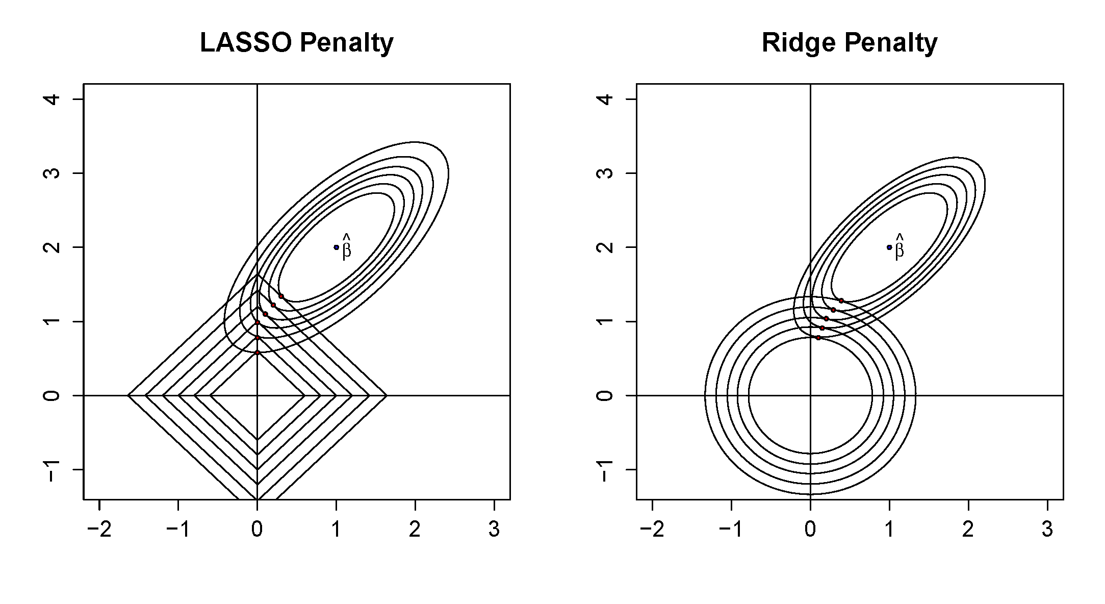
Figure 3.9: Lasso and Ridge Regression Comparison from Frees and Lee (2015)
Solution for Exercise 3.1
Exercise 3.2. Upper Limit and RVaR. For the upper limit contract, show that the range value at risk measure \(RVaR_{(\alpha,\beta)}(X \wedge u)\) is monotone increasing in \(u\).
Solution for Exercise 3.2
Exercise 3.3. Alternative Training and Testing Periods for Portfolio of Insurance Stock Returns. In this exercise, modify the set-up and code in Examples 1.1 and 3.3 to see the variation in results for alternatives training and testing periods. Specifically, the training session is a 6.5-year period, 5 January 2015 to 31 May 2021 (instead of 5 January 2015 to 31 December 2019), and the test session is a one-year period, 1 June 2020 to 31 May 2022 (instead of the three-year period 1 June 2020 to 31 May 2023). In addition to changing the relative lengths of training and test, we now consider the outlying behavior induced by the Covid epidemic.
Reproduce the results in Table 3.2 and comment on differences from those in the benchmark Table 3.1.
| Train Ann Return | Train Std Dev | Train Sharpe (Rf=0) | Test Ann Return | Test Std Dev | Test Sharpe (Rf=0) | |
|---|---|---|---|---|---|---|
| MinVar | 0.168 | 0.154 | 1.098 | 0.060 | 0.147 | 0.407 |
| Markowitz | 0.193 | 0.157 | 1.229 | 0.037 | 0.151 | 0.247 |
| Equal | 0.163 | 0.162 | 1.003 | 0.055 | 0.141 | 0.392 |
Solution for Exercise 3.3
3.6.3 Appendix. Constrained Optimization Terminology
Constrained optimization is used in many fields. So, it is natural that different sets of terminology have developed over time. Here, we set the language, or terminology, used in this book, while at the same time trying to make connections with other literatures.
- The objective function, \(f_0(\cdot)\), is a quantitative measure of the performance of the system under study that we want to minimize or maximize.
- The domain of the objective function is the set of all points \({\bf z}\) for which the function is defined.
- The objective function is a mapping of a set of characteristics to the real line. These characteristics, \({\bf z} = (z_1, \ldots, z_{p_z})^{\prime}\) are sometimes called decision variables or unknowns.
- There are typically restrictions on the decision variables through functional relationships known as constraints.
- If the constraint is of the form \(f_{con}({\bf z}) \le 0\), then it is said to be an inequality constraint.
- If the constraint is of the form \(f_{con}({\bf z}) = 0\), then it is said to be an equality constraint.
- A point is said to be feasible if it is in the domain and the constraints are satisfied.
- Optimization is the minimization or maximization of an objective function subject to constraints on its parameters.
- Our convention is to minimize an objective function \(f_0(\cdot)\). However, one can alternatively maximize \(f_0(\cdot)\) by minimizing \(-f_0(\cdot)\), so we lose no generality by focusing on minimizing functions. In economic applications one typically uses the convention of maximizing functions such as those based on the utility of resources. However, here we seek to minimize risks and costs and so use the minimization convention.
- Unconstrained optimization refers to an optimization problem where no constraints are present.
- Constrained optimization refers to an optimization problem where constraints are present.
- An optimal point, or global solution, is the point with lowest function value among all feasible points. That is, \({\bf z}^*\) is a global solution if \(f_0({\bf z}^*) \le f_0({\bf z})\) for all feasible \({\bf z}\). Note that a global solution need not be unique.
- The optimal value is the value of the objective function at a global solution.
- A local solution is a point at which the objective function is smaller than at all other feasible nearby points.
- An inequality constraint \(f_{con}({\bf z}) \le 0\) is said to be active, or binding, at \({\bf z}^*\) if \(f_{con}({\bf z}^*) = 0\).
- The term convex can be applied both to sets and to functions.
- A set \(S \in R^n\) is a convex set if the straight line segment connecting any two points in \(S\) lies entirely inside \(S\). Formally, for any two points \({\bf z}_1 \in S\) and \({\bf z}_2 \in S\), we have \(c {\bf z}_1\) \(+(1-c) {\bf z}_2\) \(\in S\) for all \(c \in [0, 1]\).
- The function \(f\) is a convex function if its domain \(S\) is a convex set and if for any two points \({\bf z}_1\) and \({\bf z}_2\) in \(S\), the following property is satisfied: \[ f(c {\bf z}_1 + (1-c) {\bf z}_2) \le cf ({\bf z}_1) + (1-c) f({\bf z}_1), \text{ for all } c \in [0, 1]. \]
- A function \(f\) is said to be concave if \(-f\) is convex.
- For a function of \(n\) variables, \(f(x_1, \ldots, x_n)\), the gradient \(\nabla f\) is its vector of first partial derivatives and the Hessian \(\nabla f ^2\) is a matrix of second partial derivatives of the form:
\[
\nabla f = \left( \begin{array}{c} \partial_{x_1} f \\ \vdots \\ \partial_{x_n} f \end{array} \right)
\ \ \ \text{and} \ \ \
\nabla ^2 f =
\left( \begin{array}{cccc}
\partial_{x_1}^2 f & \partial_{x_1, x_2} f & \cdots & \partial_{x_1, x_n} f \\
\vdots & \vdots & \ddots & \vdots \\
\partial_{x_n, x_1} f & \partial_{x_n, x_2} f & \cdots & \partial_{x_n} ^2 f \\
\end{array}
\right) .
\]
- Here, we use the short-hand notation \(\partial_{x_1} f = \frac{\partial}{\partial x_1} f\), \(\partial_{x_1}^2 f\) \(= \frac{\partial^2}{\partial x_1 ^2} f\), and \(\partial_{x_1, x_2} f\) \(= \frac{\partial^2}{\partial x_1, x_2} f\).
- A point \({\bf z}\) is stationary if its gradient is zero, that is, \(\nabla f_0({\bf z}) = 0\).
- For a multivariate function of \(n\) variables having \(m\) outcomes \((f_1, \ldots, f_m)\), the Jacobian is a matrix of first partial derivatives of the form: \[ J f = \left( \begin{array}{cccc} \partial_{x_1} f_1 & \partial_{x_2} f_1 & \cdots & \partial_{x_n} f_1 \\ \vdots & \vdots & \ddots & \vdots \\ \partial_{x_1} f_m & \partial_{x_2} f_m & \cdots & \partial_{x_n} f_m \\ \end{array} \right) . \]
3.6.4 Appendix. Designs Based on Insurance Economics
As discussed in Section 3.1, when a security loading is in place, \(\lambda_{SL} >0\), then a partial insurance coverage corresponding to a value of \(c<1\) is optimal. Schlesinger (2013) also notes that this insurance result has a portfolio interpretation. One can define \(A=w_0 - (1+\lambda_{SL}) \mathrm{E~}(y)\) to be a non-risky asset and the weighted average, \(Y(c) = (1-c) A + c (A + y)\), to be a combination of a non-risky and risky asset \(y\). In this sense, the insurance choice problem is equivalent to the portfolio problem in financial economics.
A set of related results involve the notion of a “background risk,” where the initial wealth is no longer treated as a known constant but is itself a random variable. In the portfolio context, this has a natural interpretation where \(Y(c) = (1-c) A + c (A + y)\) represents a combination of two risky assets. Typically, results on optimal coverage assume independence between two risky assets. See the review article of Schlesinger (2013) for more background and additional references.
The insurance economics approach to selection of risk retention parameters is useful but, by design, relies on individual-specific preferences. As noted by Schlesinger (2013) (page 167), “… whereas most financial assets are readily tradeable and have a risk that relates to the marketplace, insurance is a contract contingent on an individual’s personal wealth. This personal nature is what distinguishes it from other financial assets.” In contrast, this book considers instances of insurance traded from one company to another, where wealth and risk preferences play a smaller role. There is also the literature on non-optimality of the aggregate loss policy beginning with Gollier and Schlesinger (1995); see also the discussion in Gollier (2013), page 111.
3.6.5 Appendix. Designs Based on Risk Measures
As briefly introduced in Section 3.2.2, there is a vibrant literature that seeks to determine the best risk transfer designs employing risk measures to summarize uncertainty of retained risks. By and large, this literature seeks to expand the boundaries of the theory of risk retention by identifying optimal risk retention functions in conjunction with choices of risk premium principles for the cost of transferring risk and risk measures for assessing the uncertainty of retained risks. As mentioned in Section 3.2.2, these works provide insights about the types of optimal design but, due to their general nature, are difficult to implement in concrete practical settings. As remarked in Lo (2017), “In spite of the vast literature on optimal reinsurance, the majority of prior studies can be justifiably criticized for being in a vacuum detached from practicalities and externalities.” This section highlights some of the works in this literature most closely related to the ideas in this book to give readers a starting point for their own explorations into this literature.
Extending earlier work in Cai and Tan (2007), Tan and Weng (2014) utilized a constrained optimization approach, minimizing retained risk evaluated using a risk measure subject a budget constraint. Their work uses an empirical approximation of the risk retention function, thus “reducing” the problem from an infinite dimensional optimization to one involving the number of observations, a number that is large yet finite. By not imposing a specific nonlinear retention function, they were able to use convex optimization techniques to solve problems of interest.
Subsequently, this work was extended in Asimit et al. (2018) in several aspects, including considering multivariate risks. Their motivation was from an enterprise risk management perspective and so they referred to this as “multiple lines of business.” As with Tan and Weng (2014), this paper adopts an empirical approach, solving finite yet very large dimensional problems. Thus, it is not surprising that the paper restricts considerations to those problems that could be solved using convex optimization approaches. Interestingly, this paper also investigates robust optimization approaches to addressing parameter uncertainty. This topic will be taken up later in Section 9.4.
