clear all
use https://sscc.wisc.edu/~rdimond/pa871/texas8 Synthetic Control
Synthetic control is a relatively new technique that attempts to identify a mix of control observations that closely mimics the outcome of the treated observation prior to the treatment. The logic is very similar to DiD, but with an arguably stronger case for the parallel trends assumption.
Our example comes from Causal Inference: the Mixtape, and describes incarceration. Our research question: did the Texas prison building boom cause the incarceration of Black males to increase?
synth   bmprison ///
        bmprison(1990) bmprison(1992) bmprison(1991) bmprison(1988) ///
        alcohol(1990) aidscapita(1990) aidscapita(1991) ///
        income ur poverty black(1990) black(1991) black(1992) ///
        perc1519(1990), ///
        trunit(48) trperiod(1993) unitnames(state) ///
        mspeperiod(1985(1)1993) resultsperiod(1985(1)2000) ///
        keep(synth_bmprate.dta) replace fig ///
-------------------------------------------------------------------------------
Synthetic Control Method for Comparative Case Studies
-------------------------------------------------------------------------------
First Step: Data Setup
-------------------------------------------------------------------------------
-------------------------------------------------------------------------------
Data Setup successful
-------------------------------------------------------------------------------
Treated Unit: Texas
Control Units: Alabama, Alaska, Arizona, Arkansas, California,
Colorado, Connecticut, Delaware, District of
Columbia, Florida, Georgia, Hawaii, Idaho,
Illinois, Indiana, Iowa, Kansas, Kentucky,
Louisiana, Maine, Maryland, Massachusetts,
Michigan, Minnesota, Mississippi, Missouri,
Montana, Nebraska, Nevada, New Hampshire, New
Jersey, New Mexico, New York, North Carolina,
North Dakota, Ohio, Oklahoma, Oregon,
Pennsylvania, Rhode Island, South Carolina, South
Dakota, Tennessee, Utah, Vermont, Virginia,
Washington, West Virginia, Wisconsin, Wyoming
-------------------------------------------------------------------------------
Dependent Variable: bmprison
MSPE minimized for periods: 1985 1986 1987 1988 1989 1990 1991 1992 1993
Results obtained for periods: 1985 1986 1987 1988 1989 1990 1991 1992 1993 1994
1995 1996 1997 1998 1999 2000
-------------------------------------------------------------------------------
Predictors: bmprison(1990) bmprison(1992) bmprison(1991)
bmprison(1988) alcohol(1990) aidscapita(1990)
aidscapita(1991) income ur poverty black(1990)
black(1991) black(1992) perc1519(1990)
-------------------------------------------------------------------------------
Unless period is specified
predictors are averaged over: 1985 1986 1987 1988 1989 1990 1991 1992
-------------------------------------------------------------------------------
Second Step: Run Optimization
-------------------------------------------------------------------------------
-------------------------------------------------------------------------------
Optimization done
-------------------------------------------------------------------------------
Third Step: Obtain Results
-------------------------------------------------------------------------------
Loss: Root Mean Squared Prediction Error
---------------------
RMSPE | 1295.489
---------------------
-------------------------------------------------------------------------------
Unit Weights:
----------------------------------
Co_No | Unit_Weight
---------------------+------------
Alabama | 0
Alaska | 0
Arizona | 0
Arkansas | 0
California | .408
Colorado | 0
Connecticut | 0
Delaware | 0
District of Columbia | 0
Florida | .109
Georgia | 0
Hawaii | 0
Idaho | 0
Illinois | .36
Indiana | 0
Iowa | 0
Kansas | 0
Kentucky | 0
Louisiana | .122
Maine | 0
Maryland | 0
Massachusetts | 0
Michigan | 0
Minnesota | 0
Mississippi | 0
Missouri | 0
Montana | 0
Nebraska | 0
Nevada | 0
New Hampshire | 0
New Jersey | 0
New Mexico | 0
New York | 0
North Carolina | 0
North Dakota | 0
Ohio | 0
Oklahoma | 0
Oregon | 0
Pennsylvania | 0
Rhode Island | 0
South Carolina | 0
South Dakota | 0
Tennessee | 0
Utah | 0
Vermont | 0
Virginia | 0
Washington | 0
West Virginia | 0
Wisconsin | 0
Wyoming | 0
----------------------------------
-------------------------------------------------------------------------------
Predictor Balance:
------------------------------------------------------
| Treated Synthetic
-------------------------------+----------------------
bmprison(1990) | 22634 23134.8
bmprison(1992) | 27568 25776.34
bmprison(1991) | 23249 24272.24
bmprison(1988) | 16956 18374.28
alcohol(1990) | 2.47 2.70996
aidscapita(1990) | 13.58992 14.99957
aidscapita(1991) | 14.83504 17.24535
income | 16108.63 18614.54
ur | 7.426042 7.188876
poverty | 17.2 14.86484
black(1990) | 16.15459 15.98038
black(1991) | 16.29985 16.16835
black(1992) | 16.45955 16.37467
perc1519(1990) | 7.703001 7.022702
------------------------------------------------------
-------------------------------------------------------------------------------
The resulting data has been put in a file for our convenience.
clear
use synth_bmprate
l in 1/25
     +----------------------------------------------------------------+
     |           _Co_Number   _W_Wei~t   _Y_tre~d   _Y_synt~c   _time |
     |----------------------------------------------------------------|
  1. |              Alabama          0      14828   13073.971    1985 |
  2. |               Alaska          0      15207   14862.136    1986 |
  3. |              Arizona          0      15780   16206.428    1987 |
  4. |             Arkansas          0      16956    18374.28    1988 |
  5. |           California       .408      19366   21122.522    1989 |
     |----------------------------------------------------------------|
  6. |             Colorado          0      22634   23134.796    1990 |
  7. |          Connecticut          0      23249   24272.241    1991 |
  8. |             Delaware          0      27568   25776.345    1992 |
  9. | District of Columbia          0      29260   27796.861    1993 |
 10. |              Florida       .109      40451   29056.277    1994 |
     |----------------------------------------------------------------|
 11. |              Georgia          0      55602   30399.547    1995 |
 12. |               Hawaii          0      55810   31862.289    1996 |
 13. |                Idaho          0      58393   33446.808    1997 |
 14. |             Illinois        .36      59709   35026.583    1998 |
 15. |              Indiana          0      60785   35583.252    1999 |
     |----------------------------------------------------------------|
 16. |                 Iowa          0      61861   35720.355    2000 |
 17. |               Kansas          0          .           .       . |
 18. |             Kentucky          0          .           .       . |
 19. |            Louisiana       .122          .           .       . |
 20. |                Maine          0          .           .       . |
     |----------------------------------------------------------------|
 21. |             Maryland          0          .           .       . |
 22. |        Massachusetts          0          .           .       . |
 23. |             Michigan          0          .           .       . |
 24. |            Minnesota          0          .           .       . |
 25. |          Mississippi          0          .           .       . |
     +----------------------------------------------------------------+
This is an awful way to construct a data set! The first two columns describe the synthetic control, with one row per state. The last three columns describe the outcomes for real Texas and synthetic Texas, with one row per year. Never create a data set like this. If you find yourself in possession of one, fix it by splitting it into parts where rows have a consistent meaning. We’re only interested in the last three columns.
keep _Y_treated _Y_synthetic _time
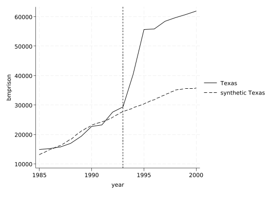
drop if _time==.(34 observations deleted)Now we can reproduce the figure synth gave us.
line _Y_synthetic _Y_treated _time, xline(1993)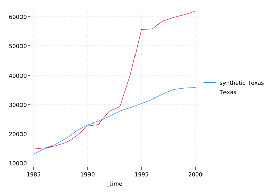
We can also create an arguably clearer graph that focuses on the difference between real Texas and synthetic Texas.
gen gap = _Y_treated - _Y_synthetic
line gap _time, xline(1993)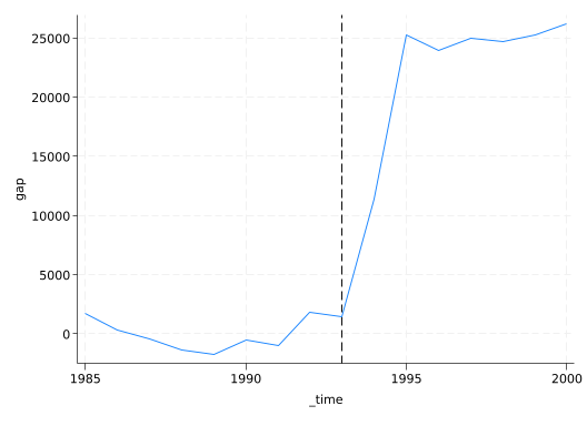
So is that gap big jump in 1993 “significant”? There’s no equivalent to a p-value here, but we can ask “How does the jump in Texas in 1993 compare to all other states?” The Mixtape has some fairly ugly code for doing so. It could be made simpler, but Brian Quistoff wrote synth_runner to do it all for you. Unfortunately it doesn’t run on Linux(!), so I can’t run it as part of this notebook (uncomment the code to run it yourself). But I can load the results and plot them.
/*
clear all
use https://sscc.wisc.edu/~rdimond/pa871/texas.dta

synth_runner    bmprison ///
        bmprison(1990) bmprison(1992) bmprison(1991) bmprison(1988) ///
        alcohol(1990) aidscapita(1990) aidscapita(1991) ///
        income ur poverty black(1990) black(1991) black(1992) ///
        perc1519(1990), ///
        trunit(48) trperiod(1993) unitnames(state) ///
        mspeperiod(1985(1)1993) gen_vars ///
        keep(synth_bmprateR.dta) replace
*/
clear
use https://sscc.wisc.edu/~rdimond/pa871/synth_bmprateR.dta
line effect year, colorvar(statefip) colordiscrete coloruseplegend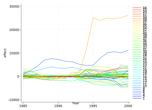
Texas very much stands out from all the other states.