clear all
use https://sscc.wisc.edu/~rdimond/pa871/gapminder.dta3 Fixed Effects
The Gapminder data contains data on countries over time. This extract contains life expectancy (life_exp) and GDP per-capita (gdp_pcap).
Cut down the sample to just 1970-2023. Also, we’re going to need a numeric code for countries rather than a string name. Finally, convert gdp_pcap to thousands of dollars just for convenience. (Interestingly, one of the later models will have convergence issues if you leave it alone or make it thousands of dollars.)
keep if year >1970 & year<2024
encode country, gen(cnum)
replace gdp_pcap = gdp_pcap/100000
(48,360 observations deleted)
(10,335 real changes made)So what does the relationship between life_exp and gdp_pcap look like?
scatter life_exp gdp_pcap if cnum<=10, colorvar(cnum) colordiscrete coloruseplegend zlabel(, valuelabel)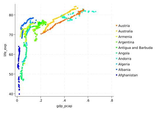
So…positive. Sort of. But the countries sure are different.
Run a regression and see what it looks like.
reg life_exp gdp_pcap
      Source |       SS           df       MS      Number of obs   =    10,335
-------------+----------------------------------   F(1, 10333)     =   4621.53
       Model |  285744.911         1  285744.911   Prob > F        =    0.0000
    Residual |  638880.396    10,333  61.8291296   R-squared       =    0.3090
-------------+----------------------------------   Adj R-squared   =    0.3090
       Total |  924625.307    10,334  89.4740959   Root MSE        =    7.8632

------------------------------------------------------------------------------
    life_exp | Coefficient  Std. err.      t    P>|t|     [95% conf. interval]
-------------+----------------------------------------------------------------
    gdp_pcap |   26.39623   .3882838    67.98   0.000     25.63512    27.15734
       _cons |   63.25835   .0977924   646.86   0.000     63.06666    63.45004
------------------------------------------------------------------------------
This ignores the differences between countries. So let’s instead treat country, or rather cnum, as a categorical variable.
reg life_exp gdp_pcap i.cnum
      Source |       SS           df       MS      Number of obs   =    10,335
-------------+----------------------------------   F(195, 10139)   =    183.11
       Model |  720137.404       195  3693.01233   Prob > F        =    0.0000
    Residual |  204487.903    10,139  20.1684488   R-squared       =    0.7788
-------------+----------------------------------   Adj R-squared   =    0.7746
       Total |  924625.307    10,334  89.4740959   Root MSE        =    4.4909

------------------------------------------------------------------------------
    life_exp | Coefficient  Std. err.      t    P>|t|     [95% conf. interval]
-------------+----------------------------------------------------------------
    gdp_pcap |   18.86835   .5390142    35.01   0.000     17.81178    19.92493
             |
        cnum |
    Albania  |   19.39616   .8729709    22.22   0.000     17.68497    21.10736
    Algeria  |   13.14916   .8732918    15.06   0.000     11.43734    14.86099
    Andorra  |   17.27633    .908471    19.02   0.000     15.49555    19.05712
     Angola  |  -.4278586    .872618    -0.49   0.624    -2.138363    1.282645
Antigua a..  |   17.56298   .8757965    20.05   0.000     15.84625    19.27972
  Argentina  |   16.01975   .8771466    18.26   0.000     14.30037    17.73913
    Armenia  |   16.42532   .8730826    18.81   0.000      14.7139    18.13673
  Australia  |   18.13644   .8923288    20.32   0.000      16.3873    19.88559
    Austria  |    16.0544   .8975558    17.89   0.000     14.29502    17.81379
 Azerbaijan  |   11.62727   .8733604    13.31   0.000      9.91531    13.33923
    Bahamas  |   11.56921   .8883778    13.02   0.000     9.827816    13.31061
    Bahrain  |     11.554   .8900366    12.98   0.000     9.809356    13.29865
 Bangladesh  |   8.483651   .8724142     9.72   0.000     6.773547    10.19376
   Barbados  |   18.04195     .87508    20.62   0.000     16.32662    19.75728
    Belarus  |   15.33128   .8741717    17.54   0.000     13.61773    17.04483
    Belgium  |   16.38781   .8948216    18.31   0.000     14.63378    18.14183
     Belize  |   17.23134   .8729014    19.74   0.000     15.52028     18.9424
      Benin  |   3.202591   .8724096     3.67   0.000     1.492496    4.912687
     Bhutan  |   8.797312   .8725871    10.08   0.000     7.086868    10.50776
    Bolivia  |   9.200655   .8726885    10.54   0.000     7.490012     10.9113
Bosnia an..  |   18.03892    .872885    20.67   0.000     16.32789    19.74995
   Botswana  |   1.835705   .8734002     2.10   0.036     .1236678    3.547742
     Brazil  |   13.08272   .8740693    14.97   0.000     11.36937    14.79607
     Brunei  |   1.922189   .9727198     1.98   0.048     .0154661    3.828913
   Bulgaria  |   14.86513   .8750536    16.99   0.000     13.14985     16.5804
Burkina F..  |  -.6780773   .8723955    -0.78   0.437    -2.388145    1.031991
    Burundi  |  -2.461115   .8724006    -2.82   0.005    -4.171193   -.7510374
   Cambodia  |   3.287071    .872403     3.77   0.000     1.576988    4.997153
   Cameroon  |   2.964247   .8724363     3.40   0.001     1.254099    4.674395
     Canada  |   17.81294   .8943288    19.92   0.000     16.05988      19.566
 Cape Verde  |    15.3489   .8724913    17.59   0.000     13.63864    17.05916
Central A..  |  -5.880191    .872398    -6.74   0.000    -7.590264   -4.170118
       Chad  |   .1890434   .8723968     0.22   0.828    -1.521027    1.899114
      Chile  |   18.08641   .8755706    20.66   0.000     16.37012     19.8027
      China  |   15.74169   .8726819    18.04   0.000     14.03106    17.45232
   Colombia  |   17.86682    .873571    20.45   0.000     16.15444    19.57919
    Comoros  |   6.702306   .8724112     7.68   0.000     4.992207    8.412405
Congo, De..  |   2.131154   .8723966     2.44   0.015     .4210843    3.841225
Congo, Rep.  |   1.816467    .872516     2.08   0.037     .1061632    3.526771
 Costa Rica  |    21.0186   .8745875    24.03   0.000     19.30424    22.73297
Cote d'Iv..  |   1.937685   .8725114     2.22   0.026     .2273901     3.64798
    Croatia  |    16.5767   .8783942    18.87   0.000     14.85488    18.29853
       Cuba  |   21.24426   .8728781    24.34   0.000     19.53325    22.95527
     Cyprus  |   16.78551   .8829116    19.01   0.000     15.05483    18.51619
Czech Rep..  |   16.11737   .8818614    18.28   0.000     14.38875      17.846
    Denmark  |   15.47935   .9003346    17.19   0.000     13.71451    17.24418
   Djibouti  |   7.526435   .8725122     8.63   0.000     5.816139    9.236732
   Dominica  |   16.52168   .8730996    18.92   0.000     14.81024    18.23313
Dominican..  |   16.20908    .873403    18.56   0.000     14.49703    17.92112
    Ecuador  |    16.3424   .8733153    18.71   0.000     14.63053    18.05427
      Egypt  |    9.69424   .8729553    11.11   0.000     7.983075    11.40541
El Salvador  |   15.09848   .8727882    17.30   0.000     13.38764    16.80932
Equatoria..  |   .4751035   .8741675     0.54   0.587    -1.238438    2.188645
    Eritrea  |   -1.33172   .8723953    -1.53   0.127    -3.041788    .3783475
    Estonia  |   14.73725   .8792051    16.76   0.000     13.01384    16.46067
   Eswatini  |   -.306678    .872661    -0.35   0.725    -2.017266     1.40391
   Ethiopia  |  -.1173925   .8723975    -0.13   0.893    -1.827464    1.592679
       Fiji  |    11.6057   .8732437    13.29   0.000     9.893966    13.31743
    Finland  |   17.07628   .8914533    19.16   0.000     15.32886    18.82371
     France  |   18.20174   .8915811    20.42   0.000     16.45406    19.94941
      Gabon  |   4.746185   .8751855     5.42   0.000     3.030648    6.461722
     Gambia  |   7.488602    .872399     8.58   0.000     5.778528    9.198677
    Georgia  |    14.5995   .8736011    16.71   0.000     12.88707    16.31193
    Germany  |   16.21532   .8953816    18.11   0.000      14.4602    17.97045
      Ghana  |   6.020424   .8724385     6.90   0.000     4.310271    7.730576
     Greece  |   19.60723   .8819433    22.23   0.000     17.87844    21.33601
    Grenada  |     15.644   .8734728    17.91   0.000     13.93182    17.35618
  Guatemala  |   9.165264   .8728548    10.50   0.000     7.454296    10.87623
     Guinea  |  -.5698511   .8723956    -0.65   0.514    -2.279919    1.140217
Guinea-Bi~u  |  -2.890927   .8723963    -3.31   0.001    -4.600996   -1.180857
     Guyana  |   8.590709    .873282     9.84   0.000     6.878904    10.30251
      Haiti  |   1.828114   .8724284     2.10   0.036     .1179817    3.538247
   Honduras  |   14.11227    .872518    16.17   0.000     12.40196    15.82257
Hong Kong..  |   12.64228   .8920455    14.17   0.000      10.8937    14.39087
    Hungary  |   14.60294   .8780538    16.63   0.000     12.88178     16.3241
    Iceland  |   18.79813   .8956019    20.99   0.000     17.04257    20.55368
      India  |   7.502909   .8724376     8.60   0.000     5.792758    9.213059
  Indonesia  |   10.36149   .8727605    11.87   0.000     8.650709    12.07228
       Iran  |   14.17784   .8742668    16.22   0.000     12.46411    15.89158
       Iraq  |   12.37067   .8729857    14.17   0.000     10.65945     14.0819
    Ireland  |   15.10982   .9009487    16.77   0.000     13.34378    16.87586
     Israel  |   19.27984   .8841218    21.81   0.000     17.54679    21.01289
      Italy  |   18.24812   .8915413    20.47   0.000     16.50053    19.99572
    Jamaica  |   19.35824   .8732728    22.17   0.000     17.64646    21.07003
      Japan  |   20.69271   .8885569    23.29   0.000     18.95096    22.43445
     Jordan  |   16.91762    .873333    19.37   0.000     15.20572    18.62953
 Kazakhstan  |   10.49616   .8759618    11.98   0.000     8.779101    12.21322
      Kenya  |   6.640893   .8724465     7.61   0.000     4.930725    8.351061
   Kiribati  |   2.480839   .8724181     2.84   0.004     .7707264    4.190951
     Kuwait  |   13.64699   .9138748    14.93   0.000     11.85561    15.43836
Kyrgyz Re..  |   12.91202   .8725633    14.80   0.000     11.20162    14.62241
        Lao  |   2.818108   .8724544     3.23   0.001     1.107925    4.528292
     Latvia  |   14.19163   .8772192    16.18   0.000     12.47211    15.91115
    Lebanon  |   15.35477   .8742995    17.56   0.000     13.64097    17.06857
    Lesotho  |  -.5317529   .8723967    -0.61   0.542    -2.241823    1.178317
    Liberia  |   1.542089   .8724078     1.77   0.077    -.1680029    3.252181
      Libya  |   15.88397   .8774943    18.10   0.000     14.16391    17.60404
  Lithuania  |   14.66823   .8784287    16.70   0.000     12.94634    16.39012
 Luxembourg  |   9.029789   .9635371     9.37   0.000     7.141066    10.91851
 Madagascar  |   4.605051   .8723958     5.28   0.000     2.894982    6.315119
     Malawi  |  -2.105175   .8723974    -2.41   0.016    -3.815246   -.3951033
   Malaysia  |   15.90489   .8753863    18.17   0.000     14.18896    17.62082
   Maldives  |   12.34994   .8740045    14.13   0.000     10.63671    14.06316
       Mali  |   -1.42439   .8723954    -1.63   0.103    -3.134458    .2856777
      Malta  |   19.71873   .8803962    22.40   0.000     17.99298    21.44449
Marshall ..  |   9.086459   .8724661    10.41   0.000     7.376253    10.79667
 Mauritania  |    8.30618    .872505     9.52   0.000     6.595897    10.01646
  Mauritius  |   15.06353   .8744272    17.23   0.000     13.34948    16.77758
     Mexico  |   14.88445   .8757381    17.00   0.000     13.16783    16.60107
Micronesi..  |   7.746696   .8724391     8.88   0.000     6.036543    9.456849
    Moldova  |   13.12574   .8735371    15.03   0.000     11.41343    14.83804
     Monaco  |   -.756888   1.126048    -0.67   0.501    -2.964164    1.450388
   Mongolia  |   6.756974   .8726943     7.74   0.000      5.04632    8.467627
 Montenegro  |   17.93205   .8751064    20.49   0.000     16.21667    19.64743
    Morocco  |   12.55594   .8726274    14.39   0.000     10.84542    14.26647
 Mozambique  |  -1.560659   .8724044    -1.79   0.074    -3.270745    .1494259
    Myanmar  |   4.216595   .8723971     4.83   0.000     2.506524    5.926666
    Namibia  |   4.618303    .873044     5.29   0.000     2.906964    6.329642
      Nauru  |   3.918531   .8788022     4.46   0.000     2.195904    5.641157
      Nepal  |   7.780663   .8724013     8.92   0.000     6.070584    9.490742
Netherlands  |   16.98445   .8982199    18.91   0.000     15.22376    18.74514
New Zealand  |   17.76939   .8878218    20.01   0.000     16.02909     19.5097
  Nicaragua  |   15.53338   .8725587    17.80   0.000     13.82299    17.24376
      Niger  |  -2.031455   .8723976    -2.33   0.020    -3.741527   -.3213826
    Nigeria  |   2.404473   .8724685     2.76   0.006     .6942618    4.114684
North Korea  |   13.13189    .872411    15.05   0.000     11.42179    14.84199
North Mac..  |   15.38226   .8741751    17.60   0.000      13.6687    17.09582
     Norway  |   16.02998   .9084795    17.64   0.000     14.24918    17.81078
       Oman  |   8.487606   .8831274     9.61   0.000     6.756501    10.21871
   Pakistan  |   7.452142   .8724537     8.54   0.000      5.74196    9.162324
      Palau  |   7.788918   .8778686     8.87   0.000     6.068122    9.509715
  Palestine  |   14.59931   .8725445    16.73   0.000     12.88895    16.30967
     Panama  |   19.84229   .8762318    22.65   0.000     18.12471    21.55988
Papua New..  |   8.534913   .8724431     9.78   0.000     6.824751    10.24507
   Paraguay  |   19.58811   .8733123    22.43   0.000     17.87624    21.29997
       Peru  |   16.93525   .8731454    19.40   0.000     15.22371    18.64678
Philippines  |   14.07535   .8726172    16.13   0.000     12.36484    15.78585
     Poland  |   16.79875   .8766829    19.16   0.000     15.08028    18.51722
   Portugal  |   17.91763   .8813093    20.33   0.000     16.19009    19.64517
      Qatar  |   3.259827   .9677443     3.37   0.001     1.362857    5.156798
    Romania  |   15.05017    .875567    17.19   0.000     13.33388    16.76645
     Russia  |   11.33477   .8776998    12.91   0.000     9.614306    13.05524
     Rwanda  |   .5265904   .8723958     0.60   0.546    -1.183478    2.236659
      Samoa  |   13.15495   .8725572    15.08   0.000     11.44456    14.86533
 San Marino  |   15.24963   .9237323    16.51   0.000     13.43893    17.06033
Sao Tome ..  |   11.02277   .8724395    12.63   0.000     9.312619    12.73293
Saudi Ara..  |   8.209762   .8972483     9.15   0.000     6.450978    9.968546
    Senegal  |   5.790201   .8724193     6.64   0.000     4.080087    7.500316
     Serbia  |   15.42711   .8748122    17.63   0.000      13.7123    17.14191
 Seychelles  |   14.64614   .8764564    16.71   0.000     12.92811    16.36417
Sierra Le..  |  -1.088042   .8723953    -1.25   0.212     -2.79811    .6220254
  Singapore  |   14.54489   .9131093    15.93   0.000     12.75501    16.33476
Slovak Re..  |   16.21032   .8774309    18.47   0.000     14.49038    17.93025
   Slovenia  |   16.93228   .8835445    19.16   0.000     15.20036     18.6642
Solomon I..  |   2.142464   .8724033     2.46   0.014     .4323806    3.852547
    Somalia  |  -2.027417   .8723986    -2.32   0.020    -3.737491   -.3173435
South Afr..  |   3.992586   .8738808     4.57   0.000     2.279607    5.705566
South Korea  |   17.20977   .8792156    19.57   0.000     15.48633    18.93321
South Sudan  |   3.023818   .8723975     3.47   0.001     1.313746    4.733889
      Spain  |   19.64801   .8850025    22.20   0.000     17.91323    21.38279
  Sri Lanka  |    16.8485   .8728322    19.30   0.000     15.13757    18.55942
St. Kitts..  |   11.33994   .8767748    12.93   0.000     9.621288    13.05859
  St. Lucia  |   16.38027   .8736387    18.75   0.000     14.66777    18.09278
St. Vince..  |   15.29897   .8732097    17.52   0.000     13.58731    17.01063
      Sudan  |   7.288347   .8724512     8.35   0.000      5.57817    8.998524
   Suriname  |   13.53323   .8751892    15.46   0.000     11.81768    15.24877
     Sweden  |   18.48339   .8946342    20.66   0.000     16.72973    20.23705
Switzerland  |   15.97752   .9163124    17.44   0.000     14.18137    17.77368
      Syria  |   15.22321   .8733157    17.43   0.000     13.51134    16.93508
     Taiwan  |   17.58298   .8827163    19.92   0.000     15.85268    19.31328
 Tajikistan  |   12.03292    .872467    13.79   0.000     10.32271    13.74313
   Tanzania  |   3.645635   .8723954     4.18   0.000     1.935567    5.355702
   Thailand  |   16.88291   .8735696    19.33   0.000     15.17054    18.59528
Timor-Leste  |   8.317864   .8724089     9.53   0.000     6.607769    10.02796
       Togo  |   4.267778   .8723962     4.89   0.000     2.557708    5.977847
      Tonga  |   16.35965   .8725161    18.75   0.000     14.64935    18.06995
Trinidad ..  |   13.54054   .8773561    15.43   0.000     11.82075    15.26033
    Tunisia  |   16.92592   .8729871    19.39   0.000      15.2147    18.63715
     Turkey  |   14.48794   .8758145    16.54   0.000     12.77117    16.20471
Turkmenis~n  |   11.00744   .8731582    12.61   0.000      9.29588    12.71901
     Tuvalu  |   8.504581   .8724449     9.75   0.000     6.794416    10.21475
        UAE  |   1.377637   .9624561     1.43   0.152    -.5089676    3.264241
         UK  |   17.14749   .8904927    19.26   0.000     15.40195    18.89303
        USA  |   14.06179   .9045857    15.55   0.000     12.28862    15.83495
     Uganda  |   .7819791   .8723953     0.90   0.370    -.9280885    2.492047
    Ukraine  |    14.4127   .8740233    16.49   0.000     12.69944    16.12596
    Uruguay  |   17.48096   .8754565    19.97   0.000      15.7649    19.19703
 Uzbekistan  |   12.32152   .8726142    14.12   0.000     10.61102    14.03202
    Vanuatu  |   9.043494   .8724225    10.37   0.000     7.333373    10.75361
  Venezuela  |   15.89228   .8760994    18.14   0.000     14.17495    17.60961
    Vietnam  |   15.30201   .8725267    17.54   0.000     13.59169    17.01234
      Yemen  |   6.324304   .8724412     7.25   0.000     4.614146    8.034461
     Zambia  |   .0177563   .8724121     0.02   0.984    -1.692344    1.727857
   Zimbabwe  |   2.543638   .8724076     2.92   0.004     .8335466     4.25373
             |
       _cons |   53.56116     .61693    86.82   0.000     52.35185    54.77046
------------------------------------------------------------------------------
Afghanistan is the first country in the data set, so the coefficients for the other countries represent the difference in life expectancy between them and Afghanistan (controlling for gdp_pcap). Most but not all are positive, and many are quite large. R-squared also increased by a lot. Clearly country is important here.
On the other hand, it sure is a lot of coefficients. If we’re just trying to get the right coefficient on gdp_pcap and we’re just controlling for country, we don’t really care about all the country coefficients. We just say we’re including country fixed effects and call it good.
The xtreg command will take care of that for us, but the data needs to be xtset so it understands the structure of the data. In particular, it needs to know the variable that identifies the countries and the variable that identifies time. Then when we tell xtreg we want fixed effects, it knows we want fixed effects for countries.
xtset cnum year
xtreg life_exp gdp_pcap, fe
Panel variable: cnum (strongly balanced)
 Time variable: year, 1971 to 2023
         Delta: 1 unit

Fixed-effects (within) regression               Number of obs     =     10,335
Group variable: cnum                            Number of groups  =        195

R-squared:                                      Obs per group:
     Within  = 0.1078                                         min =         53
     Between = 0.3822                                         avg =       53.0
     Overall = 0.3090                                         max =         53

                                                F(1, 10139)       =    1225.37
corr(u_i, Xb) = 0.2254                          Prob > F          =     0.0000

------------------------------------------------------------------------------
    life_exp | Coefficient  Std. err.      t    P>|t|     [95% conf. interval]
-------------+----------------------------------------------------------------
    gdp_pcap |   18.86835   .5390142    35.01   0.000     17.81178    19.92493
       _cons |   64.41851   .0940855   684.68   0.000     64.23408    64.60293
-------------+----------------------------------------------------------------
     sigma_u |  6.6714422
     sigma_e |  4.4909296
         rho |  .68816462   (fraction of variance due to u_i)
------------------------------------------------------------------------------
F test that all u_i=0: F(194, 10139) = 111.02                Prob > F = 0.0000
Stata refers to the fixed effects as u. So sigma_u tells us the standard deviation of the fixed effects, and rho tells us how much of the variance is explained by the fixed effects (a lot, because countries are very different). But it doesn’t report the actual coefficients.
Putting in a coefficient for each country turns out to be mathematically equivalent to calculating the mean value of all the variables for each country and then subtracting it from all the values for that country. Thus the model only looks at the variation over time within each country in estimating the effect of life_exp. Note that this means you can’t include any predictors that don’t change over time in a fixed effects model. The model can’t tell the difference between a variable that’s always the same for a country and the effect of the country itself.
An obvious problem with this regression is that per-capita GDP usually increases over time, and lots of other things change over time. So some of the effect we observe for gdp_pcap could actually be due to other things that change over time. So let’s include time in the model but what’s the form of the relationship? To see, graph the mean of life_exp by year.
graph bar (mean) life_exp, over(year)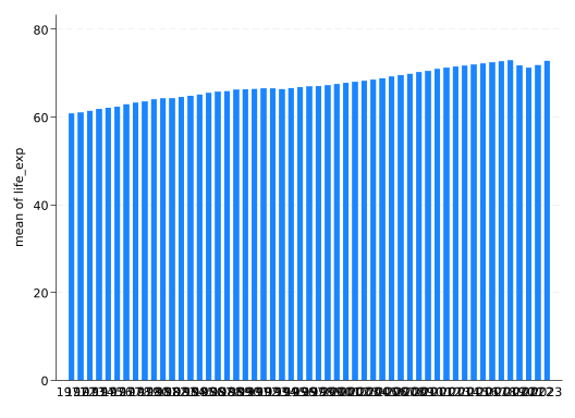
Well that’s not very useful! This is why your default for bar graphs should be horizontal.
graph hbar (mean) life_exp, over(year, label(labsize(vsmall)))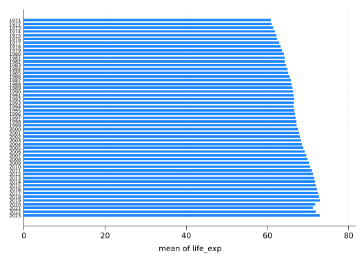
The relationship is not all that linear–and then we’ve got the COVID-19 pandemic at the end. So rather than treating year as a continuous variable and assuming a linear relationship with life_exp, let’s add fixed effects for time too. xtreg only does fixed effects for each subject automatically, but we can tell it to absorb the year variable, which essentially means put in i.year without reporting coefficients for it.
xtreg life_exp gdp_pcap, fe absorb(year)
Halperin APM for regression coefficients:

Dependent variable:
Iteration 1:  Maximum absolute difference = 2.109e-13

Independent variables:
Iteration 1:  Maximum absolute difference = 2.057e-14

Halperin APM for panel effects:
Iteration 1:  Maximum absolute difference =     13.22
Iteration 2:  Maximum absolute difference = 6.402e-15

Fixed-effects (within) regression               Number of obs     =     10,335
Group variable: cnum                            Number of groups  =        195

R-squared:                                      Obs per group:
     Within  = 0.5373                                         min =         53
     Between = 0.3822                                         avg =       53.0
     Overall = 0.3090                                         max =         53

                                                F(1, 10087)       =       1.87
corr(u_i, Xb) = -0.5709                         Prob > F          =     0.1711

--------------------------
Absorbed variable | Levels
------------------+-------
             year |     53
--------------------------
------------------------------------------------------------------------------
    life_exp | Coefficient  Std. err.      t    P>|t|     [95% conf. interval]
-------------+----------------------------------------------------------------
    gdp_pcap |  -.6062292   .4429366    -1.37   0.171    -1.474473    .2620147
       _cons |   67.41982   .0753466   894.80   0.000     67.27213    67.56752
-------------+----------------------------------------------------------------
     sigma_u |   8.292725
     sigma_e |  3.2424726
         rho |    .867391   (fraction of variance due to u_i)
------------------------------------------------------------------------------
F test that all u_i=0: F(194, 10087) = 261.24                Prob > F = 0.0000
After controlling for time and country gdp_pcap has no effect on life_exp. Do you believe that? Not without checking model diagnostics!
There are several different ways you can calculate the predicted values for a fixed effect model, so you can’t just use rvfplot. We want to include the fixed effects in calculating the predicted values and use the individual-level error in looking at residuals.
predict life_exp_hat, xbu
predict residual, e
Halperin APM for panel effects:
Iteration 1:  Maximum absolute difference =     13.22
Iteration 2:  Maximum absolute difference = 6.402e-15

Halperin APM for absorbed effects:
Iteration 1:  Maximum absolute difference = 3.400e-13
scatter residual life_exp_hat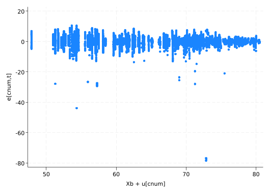
scatter residual gdp_pcap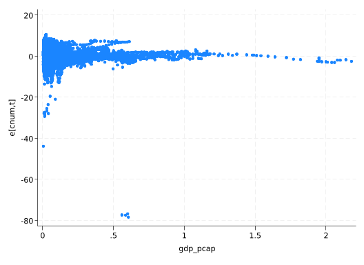
The downward trend is a bit concerning, as is the fact that there are some big negative residuals but no corresponding big positive residuals.
hist residual(bin=40, start=-78.38623, width=2.2226786)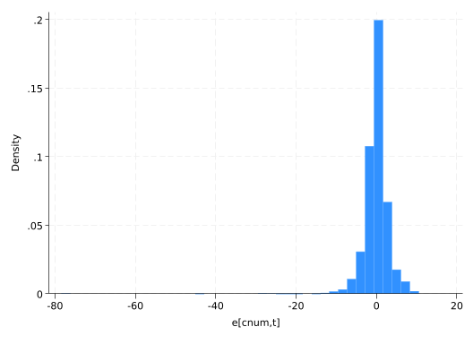
Take a closer look without the big negative residuals.
hist residual if residual>-15(bin=40, start=-14.741642, width=.63156393)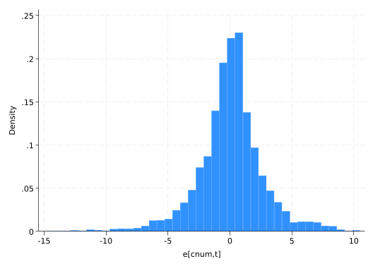
qnorm residual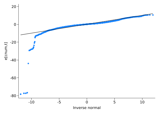
So all admirably normal, except for those big negative residuals. What’s up with those?
list country year life_exp gdp_pcap residual if residual<-15
       +-----------------------------------------------------------+
       |          country   year   life_exp   gdp_pcap    residual |
       |-----------------------------------------------------------|
 1433. |          Burundi   1972       17.1     .00936   -27.77646 |
 1489. |         Cambodia   1975       24.7      .0131   -27.31961 |
 1490. |         Cambodia   1976       24.5       .014   -27.74986 |
 1491. |         Cambodia   1977       24.4      .0138   -28.41938 |
 1492. |         Cambodia   1978       24.2      .0149   -28.91995 |
       |-----------------------------------------------------------|
 1493. |         Cambodia   1979       24.1      .0142   -29.30515 |
 2336. |           Cyprus   1974         49      .0898   -20.94798 |
 3856. |            Haiti   2010       32.5      .0294   -26.58132 |
 3972. | Hong Kong, China   2020          0       .559   -77.32952 |
 3973. | Hong Kong, China   2021          0         .6    -76.7635 |
       |-----------------------------------------------------------|
 3974. | Hong Kong, China   2022          0       .585   -77.43473 |
 3975. | Hong Kong, China   2023          0       .605   -78.38623 |
 4988. |          Lebanon   1976       38.3      .0403   -27.95316 |
 4994. |          Lebanon   1982       48.6      .0526   -19.52872 |
 6999. |        Palestine   1973       37.6      .0294   -25.46058 |
       |-----------------------------------------------------------|
 7008. |        Palestine   1982       42.3      .0382    -23.5813 |
 7603. |           Rwanda   1994        9.5     .00539   -43.86348 |
       +-----------------------------------------------------------+
Oh…it’s civil wars, invasions, the Khmer Rouge, and the Haiti earthquake. Except for Hong Kong. Presumably once Hong Kong was returned to China they couldn’t get separate life expectancy data, but that should be missing not zero! Fix that and run the model again.
replace life_exp = . if life_exp==0(4 real changes made, 4 to missing)xtreg life_exp gdp_pcap, fe absorb(year)
Halperin APM for regression coefficients:

Dependent variable:
Iteration 1:  Maximum absolute difference =   .001916
Iteration 2:  Maximum absolute difference = 5.736e-10

Independent variables:
Iteration 1:  Maximum absolute difference = .00002363
Iteration 2:  Maximum absolute difference = 2.138e-12

Halperin APM for panel effects:
Iteration 1:  Maximum absolute difference =     13.02
Iteration 2:  Maximum absolute difference =     .4017
Iteration 3:  Maximum absolute difference =  .0001555
Iteration 4:  Maximum absolute difference = 6.017e-08
Iteration 5:  Maximum absolute difference = 2.329e-11

Fixed-effects (within) regression               Number of obs     =     10,331
Group variable: cnum                            Number of groups  =        195

R-squared:                                      Obs per group:
     Within  = 0.6125                                         min =         49
     Between = 0.3839                                         avg =       53.0
     Overall = 0.3226                                         max =         53

                                                F(1, 10083)       =       1.25
corr(u_i, Xb) = 0.5593                          Prob > F          =     0.2634

--------------------------
Absorbed variable | Levels
------------------+-------
             year |     53
--------------------------
------------------------------------------------------------------------------
    life_exp | Coefficient  Std. err.      t    P>|t|     [95% conf. interval]
-------------+----------------------------------------------------------------
    gdp_pcap |   .4305647   .3849346     1.12   0.263    -.3239838    1.185113
       _cons |   67.28618   .0654109  1028.67   0.000     67.15796     67.4144
-------------+----------------------------------------------------------------
     sigma_u |  8.2109465
     sigma_e |  2.8147619
         rho |   .8948418   (fraction of variance due to u_i)
------------------------------------------------------------------------------
F test that all u_i=0: F(194, 10083) = 347.50                Prob > F = 0.0000
That changed the sign, but the effect is still insignificant.
You may recall that the original example in The Effect uses the log of per-capita GDP. The curvature of the log function adds some diminishing returns to the model, which makes sense intuitively. So we’ll try that and see what we think is the better model. But before we do, let’s get the AIC and BIC for this model.
estat ic
Akaike's information criterion and Bayesian information criterion

-----------------------------------------------------------------------------
       Model |          N   ll(null)  ll(model)      df        AIC        BIC
-------------+---------------------------------------------------------------
           . |     10,331  -30121.55  -25224.86       2   50453.73   50468.21
-----------------------------------------------------------------------------
Note: BIC uses N = number of observations. See [R] IC note.
gen log_gdp_pcap = log(gdp_pcap)Start by looking at a scatterplot again.
scatter life_exp log_gdp_pcap if cnum<=10, colorvar(cnum) colordiscrete coloruseplegend zlabel(, valuelabel)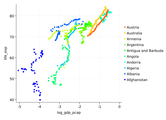
The relationship between life_exp and log_gdp_pcap does seems a little more consistent between countries, but that’s not much of a check.
xtreg life_exp log_gdp_pcap, fe absorb(year)
Halperin APM for regression coefficients:

Dependent variable:
Iteration 1:  Maximum absolute difference =   .001916
Iteration 2:  Maximum absolute difference = 5.736e-10

Independent variables:
Iteration 1:  Maximum absolute difference =  .0001471
Iteration 2:  Maximum absolute difference = 3.214e-12

Halperin APM for panel effects:
Iteration 1:  Maximum absolute difference =      10.4
Iteration 2:  Maximum absolute difference =     .3452
Iteration 3:  Maximum absolute difference =  .0001336
Iteration 4:  Maximum absolute difference = 5.172e-08
Iteration 5:  Maximum absolute difference = 2.002e-11

Fixed-effects (within) regression               Number of obs     =     10,331
Group variable: cnum                            Number of groups  =        195

R-squared:                                      Obs per group:
     Within  = 0.6289                                         min =         49
     Between = 0.7367                                         avg =       53.0
     Overall = 0.6470                                         max =         53

                                                F(1, 10083)       =     447.11
corr(u_i, Xb) = 0.7154                          Prob > F          =     0.0000

--------------------------
Absorbed variable | Levels
------------------+-------
             year |     53
--------------------------
------------------------------------------------------------------------------
    life_exp | Coefficient  Std. err.      t    P>|t|     [95% conf. interval]
-------------+----------------------------------------------------------------
log_gdp_pcap |   1.931591   .0913496    21.15   0.000     1.752527    2.110654
       _cons |   72.26024   .2336777   309.23   0.000     71.80219     72.7183
-------------+----------------------------------------------------------------
     sigma_u |  6.4687092
     sigma_e |  2.7545267
         rho |  .84650679   (fraction of variance due to u_i)
------------------------------------------------------------------------------
F test that all u_i=0: F(194, 10083) = 165.41                Prob > F = 0.0000
Now we’ve got a strong effect for log_gdp_pcap. But we still won’t believe it without diagnostics.
predict life_exp_hat2, xbu
predict residual2, e
Halperin APM for panel effects:
Iteration 1:  Maximum absolute difference =      10.4
Iteration 2:  Maximum absolute difference =     .3452
Iteration 3:  Maximum absolute difference =  .0001336
Iteration 4:  Maximum absolute difference = 5.172e-08
Iteration 5:  Maximum absolute difference = 2.002e-11
(4 missing values generated)

Halperin APM for absorbed effects:
Iteration 1:  Maximum absolute difference =    .00178
Iteration 2:  Maximum absolute difference = 7.055e-11
(4 missing values generated)
scatter residual2 life_exp_hat2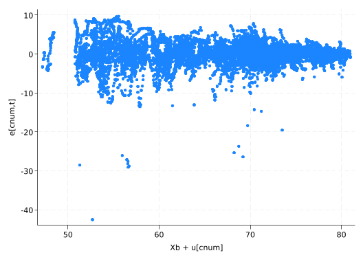
scatter residual2 log_gdp_pcap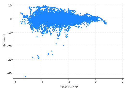
There’s somewhat less of a trend, except at the very far right end, so that’s good.
hist residual2(bin=40, start=-42.537064, width=1.3056776)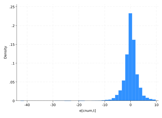
hist residual2 if residual2>-15(bin=40, start=-14.727797, width=.61044588)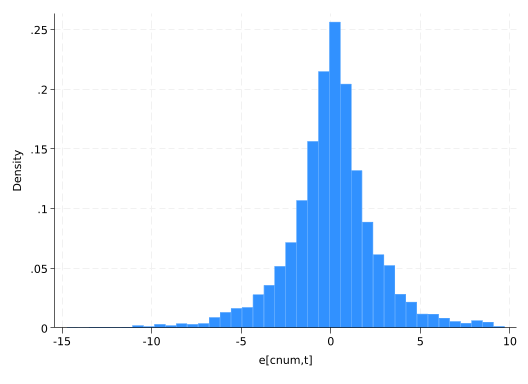
These graphs don’t make it easy to choose, so how about the information criteria?
estat ic
Akaike's information criterion and Bayesian information criterion

-----------------------------------------------------------------------------
       Model |          N   ll(null)  ll(model)      df        AIC        BIC
-------------+---------------------------------------------------------------
           . |     10,331  -30121.55  -25001.38       2   50006.76   50021.25
-----------------------------------------------------------------------------
Note: BIC uses N = number of observations. See [R] IC note.
It’s not a big difference, but both AIC and BIC are lower for the model with log_gdp_pcap, suggesting that’s the better model.