clear all
use https://sscc.wisc.edu/~rdimond/pa871/gov_transfers.dta5 Regression Discontinuity
Manacorda, Miguel, and Vigorito estimated the effect of receiving an anti-poverty payment on support for the government providing the payments by looking at how support for the government changes as income rises from just below the threshold for eligibility to just above.
We’ll start by breaking the data into “bins” by income and looking at mean support across bins.
egen income_bin = cut(income_centered), at(-.02(.001).02)
bysort income_bin: egen support_mean = mean(support)
line support_mean income_centered, sort xline(0)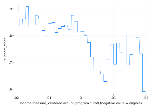
An alternative is lowess, that fits polynomial regressions at each point nearby points heavily weighted. That bandwidth makes a huge difference.
lowess support income_centered, bw(1) xline(0)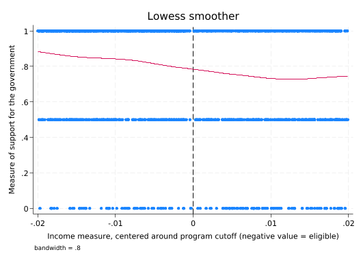
lowess support income_centered, bw(.1) xline(0)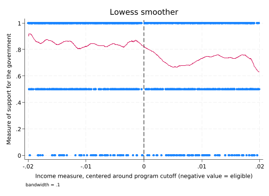
lowess support income_centered, bw(.01) xline(0)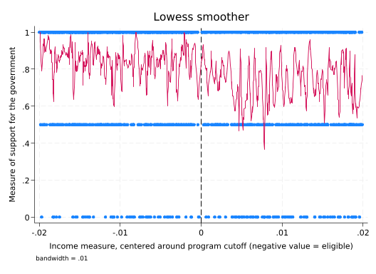
The basic vesion of regression discontinuity regresses support on participation interacted with income_centered. Thus allows participation to cause both a jump (the discontinuity) and a change in slope.
reg support participation##c.income_centered
      Source |       SS           df       MS      Number of obs   =     1,948
-------------+----------------------------------   F(3, 1944)      =     22.95
       Model |  6.74275421         3  2.24758474   Prob > F        =    0.0000
    Residual |  190.349135     1,944  .097916222   R-squared       =    0.0342
-------------+----------------------------------   Adj R-squared   =    0.0327
       Total |  197.091889     1,947    .1012285   Root MSE        =    .31292

------------------------------------------------------------------------------
     support | Coefficient  Std. err.      t    P>|t|     [95% conf. interval]
-------------+----------------------------------------------------------------
participat~n |
Got a tra..  |   .0998519   .0295488     3.38   0.001     .0419013    .1578025
income_cen~d |   -.179431   1.916171    -0.09   0.925    -3.937397    3.578535
             |
participat~n#|
          c. |
income_cen~d |
Got a tra..  |  -1.442047    2.51643    -0.57   0.567    -6.377232    3.493137
             |
       _cons |   .7296172   .0225384    32.37   0.000     .6854153    .7738191
------------------------------------------------------------------------------
Margins is not the right tool for looking at this because it treats participation as independent of income_centered. Instead, get predicted values and plot them.
predict support_hat(option xb assumed; fitted values)scatter support_hat income_centered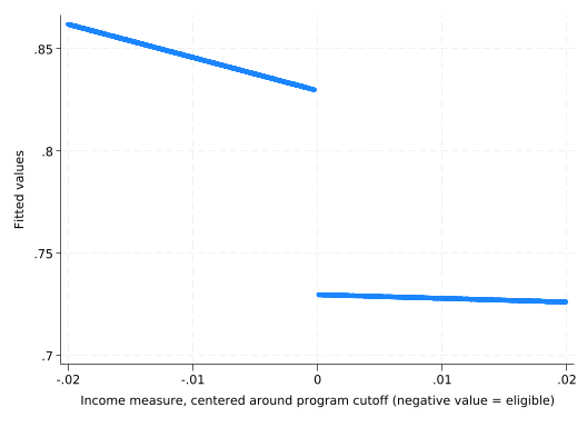
But what if it’s not a straight line? We can add income_centered squared as a predictor with an interaction.
reg support income_centered participation##c.income_centered##c.income_centerednote: income_centered omitted because of collinearity.
Source | SS df MS Number of obs = 1,948
-------------+---------------------------------- F(5, 1942) = 14.63
Model | 7.15220584 5 1.43044117 Prob > F = 0.0000
Residual | 189.939683 1,942 .097806222 R-squared = 0.0363
-------------+---------------------------------- Adj R-squared = 0.0338
Total | 197.091889 1,947 .1012285 Root MSE = .31274
------------------------------------------------------------------------------
support | Coefficient Std. err. t P>|t| [95% conf. interval]
-------------+----------------------------------------------------------------
income_cen~d | -11.56663 7.777289 -1.49 0.137 -26.81934 3.686081
|
participat~n |
Got a tra.. | .0928553 .0458508 2.03 0.043 .0029334 .1827773
income_cen~d | 0 (omitted)
|
participat~n#|
c. |
income_cen~d |
Got a tra.. | 19.29999 10.44517 1.85 0.065 -1.184931 39.7849
|
c. |
income_cen~d#|
c. |
income_cen~d | 562.2473 372.1824 1.51 0.131 -167.6717 1292.166
|
participat~n#|
c. |
income_cen~d#|
c. |
income_cen~d |
Got a tra.. | -101.1025 500.1956 -0.20 0.840 -1082.079 879.8742
|
_cons | .7689957 .0344512 22.32 0.000 .7014305 .8365609
------------------------------------------------------------------------------predict support_hat2(option xb assumed; fitted values)scatter support_hat2 income_centered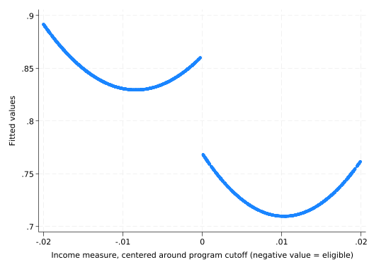
Note that any time you estimate a polynomial of degree greater than 1, the extremes are going to be the least precisely estimated–but that’s what RD relies on.
Regression discontinuity is often done with weights: points closer to the threshold count for more. A popular version is simply a triangle.
gen weight = 1 - 100*abs(income_centered)
replace weight = 0 if weight < 0
(1,011 real changes made)scatter weight income_centered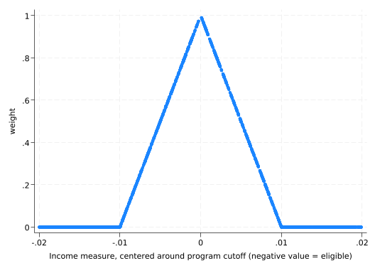
With these weights we’re ignoring points further than .01 from the threshold.
reg support participation##c.income_centered [aw=weight], robust(sum of wgt is 459.9937024153769)
Linear regression Number of obs = 937
F(3, 933) = 12.92
Prob > F = 0.0000
R-squared = 0.0415
Root MSE = .30909
------------------------------------------------------------------------------
| Robust
support | Coefficient std. err. t P>|t| [95% conf. interval]
-------------+----------------------------------------------------------------
participat~n |
Got a tra.. | .0334818 .0441959 0.76 0.449 -.0532531 .1202166
income_cen~d | -23.69669 6.680465 -3.55 0.000 -36.80717 -10.58621
|
participat~n#|
c. |
income_cen~d |
Got a tra.. | 26.59367 9.198351 2.89 0.004 8.541818 44.64553
|
_cons | .8194073 .0321537 25.48 0.000 .7563053 .8825094
------------------------------------------------------------------------------rdrobust does this all this for us.
rdrobust support income_centeredMass points detected in the running variable.
Sharp RD estimates using local polynomial regression.
Cutoff c = 0 | Left of c Right of c Number of obs = 194
> 8
-------------------+---------------------- BW type = mser
> d
Number of obs | 1127 821 Kernel = Triangula
> r
Eff. Number of obs | 291 194 VCE method = N
> N
Order est. (p) | 1 1
Order bias (q) | 2 2
BW est. (h) | 0.005 0.005
BW bias (b) | 0.010 0.010
rho (h/b) | 0.509 0.509
Unique obs | 841 639
Outcome: support. Running variable: income_centered.
-------------------------------------------------------------------------------
> -
Method | Coef. Std. Err. z P>|z| [95% Conf. Interval
> ]
-------------------+-----------------------------------------------------------
> -
Conventional | .0247 .06236 0.3961 0.692 -.09752 .14692
> 4
Robust | - - 0.6238 0.533 -.097391 .18832
> 5
-------------------------------------------------------------------------------
> -
Estimates adjusted for mass points in the running variable.rdrobust tries to select the best bandwidth. But the data was selected to be very close to the threshold, so it’s not clear weighting is needed. A bandwidth that’s a good bit bigger than the actual span of the data will get pretty much the results we had before. Set it with the h() option.
rdrobust support income_centered, h(100)
Sharp RD estimates using local polynomial regression.

      Cutoff c = 0 | Left of c  Right of c            Number of obs =       194
> 8
-------------------+----------------------            BW type       =     Manua
> l
     Number of obs |      1127         821            Kernel        = Triangula
> r
Eff. Number of obs |      1127         821            VCE method    =         N
> N
    Order est. (p) |         1           1
    Order bias (q) |         2           2
       BW est. (h) |   100.000     100.000
       BW bias (b) |   100.000     100.000
         rho (h/b) |     1.000       1.000

Outcome: support. Running variable: income_centered.
-------------------------------------------------------------------------------
> -
            Method |   Coef.    Std. Err.    z     P>|z|    [95% Conf. Interval
> ]
-------------------+-----------------------------------------------------------
> -
      Conventional | -.09985     .02967   -3.3658  0.001   -.157996     -.04170
> 7
            Robust |     -          -     -2.1585  0.031   -.177161     -.00854
> 1
-------------------------------------------------------------------------------
> -
We can use polynomials with the p() option. rdplot will show us what that looks like.
rdplot support income_centered, p(1)Mass points detected in the running variable.
RD Plot with evenly spaced mimicking variance number of bins using polynomial r
> egression.
Cutoff c = 0 | Left of c Right of c Number of obs = 194
> 8
----------------------+---------------------- Kernel = Unifor
> m
Number of obs | 1127 821
Eff. Number of obs | 1126 820
Order poly. fit (p) | 1 1
BW poly. fit (h) | 0.020 0.020
Number of bins scale | 1.000 1.000
Outcome: support. Running variable: income_centered.
---------------------------------------------
| Left of c Right of c
----------------------+----------------------
Bins selected | 35 35
Average bin length | 0.001 0.001
Median bin length | 0.001 0.001
----------------------+----------------------
IMSE-optimal bins | 3 7
Mimicking Var. bins | 35 35
----------------------+----------------------
Rel. to IMSE-optimal: |
Implied scale | 11.667 5.000
WIMSE var. weight | 0.001 0.008
WIMSE bias weight | 0.999 0.992
---------------------------------------------

rdplot support income_centered, p(2)Mass points detected in the running variable.
RD Plot with evenly spaced mimicking variance number of bins using polynomial r
> egression.
Cutoff c = 0 | Left of c Right of c Number of obs = 194
> 8
----------------------+---------------------- Kernel = Unifor
> m
Number of obs | 1127 821
Eff. Number of obs | 1126 820
Order poly. fit (p) | 2 2
BW poly. fit (h) | 0.020 0.020
Number of bins scale | 1.000 1.000
Outcome: support. Running variable: income_centered.
---------------------------------------------
| Left of c Right of c
----------------------+----------------------
Bins selected | 35 35
Average bin length | 0.001 0.001
Median bin length | 0.001 0.001
----------------------+----------------------
IMSE-optimal bins | 3 7
Mimicking Var. bins | 35 35
----------------------+----------------------
Rel. to IMSE-optimal: |
Implied scale | 11.667 5.000
WIMSE var. weight | 0.001 0.008
WIMSE bias weight | 0.999 0.992
---------------------------------------------
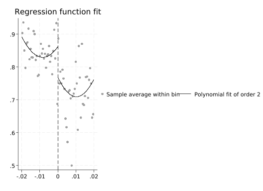
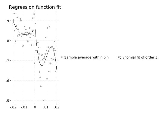
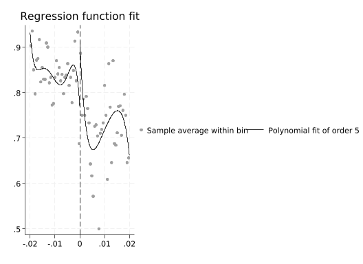
Higher order polynomials tend to wiggle around to capture random noise in the data: “overfitting”.
rdplot support income_centered, p(3)Mass points detected in the running variable.
RD Plot with evenly spaced mimicking variance number of bins using polynomial r
> egression.
Cutoff c = 0 | Left of c Right of c Number of obs = 194
> 8
----------------------+---------------------- Kernel = Unifor
> m
Number of obs | 1127 821
Eff. Number of obs | 1126 820
Order poly. fit (p) | 3 3
BW poly. fit (h) | 0.020 0.020
Number of bins scale | 1.000 1.000
Outcome: support. Running variable: income_centered.
---------------------------------------------
| Left of c Right of c
----------------------+----------------------
Bins selected | 35 35
Average bin length | 0.001 0.001
Median bin length | 0.001 0.001
----------------------+----------------------
IMSE-optimal bins | 3 7
Mimicking Var. bins | 35 35
----------------------+----------------------
Rel. to IMSE-optimal: |
Implied scale | 11.667 5.000
WIMSE var. weight | 0.001 0.008
WIMSE bias weight | 0.999 0.992
---------------------------------------------
rdplot support income_centered, p(4)Mass points detected in the running variable.
RD Plot with evenly spaced mimicking variance number of bins using polynomial r
> egression.
Cutoff c = 0 | Left of c Right of c Number of obs = 194
> 8
----------------------+---------------------- Kernel = Unifor
> m
Number of obs | 1127 821
Eff. Number of obs | 1126 820
Order poly. fit (p) | 4 4
BW poly. fit (h) | 0.020 0.020
Number of bins scale | 1.000 1.000
Outcome: support. Running variable: income_centered.
---------------------------------------------
| Left of c Right of c
----------------------+----------------------
Bins selected | 35 35
Average bin length | 0.001 0.001
Median bin length | 0.001 0.001
----------------------+----------------------
IMSE-optimal bins | 3 7
Mimicking Var. bins | 35 35
----------------------+----------------------
Rel. to IMSE-optimal: |
Implied scale | 11.667 5.000
WIMSE var. weight | 0.001 0.008
WIMSE bias weight | 0.999 0.992
---------------------------------------------

rdplot support income_centered, p(5)Mass points detected in the running variable.
RD Plot with evenly spaced mimicking variance number of bins using polynomial r
> egression.
Cutoff c = 0 | Left of c Right of c Number of obs = 194
> 8
----------------------+---------------------- Kernel = Unifor
> m
Number of obs | 1127 821
Eff. Number of obs | 1126 820
Order poly. fit (p) | 5 5
BW poly. fit (h) | 0.020 0.020
Number of bins scale | 1.000 1.000
Outcome: support. Running variable: income_centered.
---------------------------------------------
| Left of c Right of c
----------------------+----------------------
Bins selected | 35 35
Average bin length | 0.001 0.001
Median bin length | 0.001 0.001
----------------------+----------------------
IMSE-optimal bins | 3 7
Mimicking Var. bins | 35 35
----------------------+----------------------
Rel. to IMSE-optimal: |
Implied scale | 11.667 5.000
WIMSE var. weight | 0.001 0.008
WIMSE bias weight | 0.999 0.992
---------------------------------------------
rdplot support income_centered, p(6)Mass points detected in the running variable.
RD Plot with evenly spaced mimicking variance number of bins using polynomial r
> egression.
Cutoff c = 0 | Left of c Right of c Number of obs = 194
> 8
----------------------+---------------------- Kernel = Unifor
> m
Number of obs | 1127 821
Eff. Number of obs | 1126 820
Order poly. fit (p) | 6 6
BW poly. fit (h) | 0.020 0.020
Number of bins scale | 1.000 1.000
Outcome: support. Running variable: income_centered.
---------------------------------------------
| Left of c Right of c
----------------------+----------------------
Bins selected | 35 35
Average bin length | 0.001 0.001
Median bin length | 0.001 0.001
----------------------+----------------------
IMSE-optimal bins | 3 7
Mimicking Var. bins | 35 35
----------------------+----------------------
Rel. to IMSE-optimal: |
Implied scale | 11.667 5.000
WIMSE var. weight | 0.001 0.008
WIMSE bias weight | 0.999 0.992
---------------------------------------------
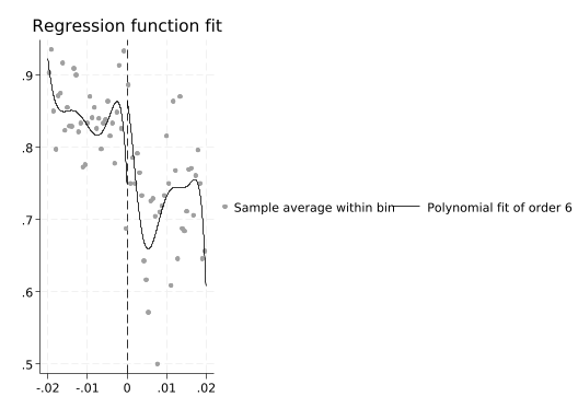
Note how the discontinuity at 0 changes radically! Don’t do that.