clear all
webuse cattaneo2
(Excerpt from Cattaneo (2010) Journal of Econometrics 155: 138–154)Propensity score matching was very popular 10-15 years ago. But the more people dug into it the more complicated it became. Then King & Nielson went and wrote their well-titled paper Why Propensity Scores Should Not Be Used for Matching. But you’ll still see a lot of it.
The cattaneo2 data set (used in Stata’s documentation and thus available via webuse) contains data on women’s pregnancy outcomes. The question at hand: does smoking during pregnancy lower birth weight?
clear all
webuse cattaneo2(Excerpt from Cattaneo (2010) Journal of Econometrics 155: 138–154)There’s certain a difference.
tab mbsmoke, sum(bweight)
            |    Summary of Infant birthweight
1 if mother |               (grams)
     smoked |        Mean   Std. dev.       Freq.
------------+------------------------------------
  Nonsmoker |   3412.9116   570.68711       3,778
     Smoker |   3137.6597   560.89305         864
------------+------------------------------------
      Total |   3361.6799   578.81962       4,642
But smoking is hardly a randomly assigned treatment, and women who smoked during pregnancy are different in many variables that could plausibly predict low birth weight.
table () (mbsmoke), stat(mean mage medu prenatal1 alcohol) nototal
----------------------------------------------------------------
                                         |   1 if mother smoked
                                         |  Nonsmoker     Smoker
-----------------------------------------+----------------------
Mother's age                             |   26.81048   25.16667
Mother's education attainment            |   12.92986   11.63889
1 if first prenatal visit in 1 trimester |   .8268925   .6898148
1 if alcohol consumed during pregnancy   |    .018793   .0914352
----------------------------------------------------------------
We could just run a regression.
reg bweight mbsmoke mage medu prenatal1 alcohol
      Source |       SS           df       MS      Number of obs   =     4,642
-------------+----------------------------------   F(5, 4636)      =     45.28
       Model |  72403839.6         5  14480767.9   Prob > F        =    0.0000
    Residual |  1.4825e+09     4,636  319775.754   R-squared       =    0.0466
-------------+----------------------------------   Adj R-squared   =    0.0455
       Total |  1.5549e+09     4,641  335032.156   Root MSE        =    565.49

------------------------------------------------------------------------------
     bweight | Coefficient  Std. err.      t    P>|t|     [95% conf. interval]
-------------+----------------------------------------------------------------
     mbsmoke |  -237.8576   22.10275   -10.76   0.000    -281.1895   -194.5257
        mage |   6.070666   1.642302     3.70   0.000     2.850972    9.290359
        medu |   8.839124   3.718692     2.38   0.017     1.548719    16.12953
   prenatal1 |   75.92022   22.01598     3.45   0.001     32.75842     119.082
     alcohol |  -77.05216   47.73211    -1.61   0.107    -170.6298    16.52548
       _cons |   3074.536   50.88495    60.42   0.000     2974.777    3174.294
------------------------------------------------------------------------------
But getting a regression model right is hard (all those diagnostics) so matching seems like an appealing alternative. The trouble is finding a good way to identify matches. Propensity score matching suggests matching observations with similar probabilities of being treated. This is not really about controlling for how treatment got assigned. Rather, it’s a measure of similarity that’s directly relevant to what we care about.
To estimate the probability of treatment we use a logit model. (So much for avoiding regression!)
logit mbsmoke mage medu prenatal1 alcohol
Iteration 0:  Log likelihood = -2230.7484
Iteration 1:  Log likelihood = -2096.3036
Iteration 2:  Log likelihood = -2086.3683
Iteration 3:  Log likelihood = -2086.3204
Iteration 4:  Log likelihood = -2086.3204

Logistic regression                                     Number of obs =  4,642
                                                        LR chi2(4)    = 288.86
                                                        Prob > chi2   = 0.0000
Log likelihood = -2086.3204                             Pseudo R2     = 0.0647

------------------------------------------------------------------------------
     mbsmoke | Coefficient  Std. err.      z    P>|z|     [95% conf. interval]
-------------+----------------------------------------------------------------
        mage |  -.0211329   .0075059    -2.82   0.005    -.0358442   -.0064216
        medu |  -.1585844   .0165668    -9.57   0.000    -.1910547   -.1261141
   prenatal1 |   -.382945   .0931037    -4.11   0.000    -.5654249   -.2004651
     alcohol |   1.621586   .1757901     9.22   0.000     1.277044    1.966128
       _cons |   1.247558   .2239144     5.57   0.000     .8086939    1.686422
------------------------------------------------------------------------------
While we could proceed to get the predicted values and then find the matches ourselves, far better to let Stata take care of all that and just give us the treatment effect in the end.
teffects psmatch (bweight) (mbsmoke mage medu prenatal1 alcohol)
Treatment-effects estimation                   Number of obs      =      4,642
Estimator      : propensity-score matching     Matches: requested =          1
Outcome model  : matching                                     min =          1
Treatment model: logit                                        max =        116
------------------------------------------------------------------------------
             |              AI robust
     bweight | Coefficient  std. err.      z    P>|z|     [95% conf. interval]
-------------+----------------------------------------------------------------
ATE          |
     mbsmoke |
    (Smoker  |
         vs  |
 Nonsmoker)  |  -219.6847   28.67382    -7.66   0.000    -275.8844   -163.4851
------------------------------------------------------------------------------
This is within a standard error of our regression results. But do we trust it? Not without diagnostics.
Propensity score matching only works if all observations have some probability of being either treated or not treated. This is called the overlap assumption because the distributions of the propensity scores need to overlap.
teoverlap(refitting the model using the generate() option)
Of course they won’t fully overlap (unless our treatment model has no predictive power) but there’s a lot of overlap and no spikes right by 0 or 1.
The next question is whether the matching actually made the treated group and the control group more balanced. To see how the treatment model affects balance, start with a simpler model.
teffects psmatch (bweight) (mbsmoke medu)
tebalance summarize mage medu prenatal1 alcohol
Treatment-effects estimation                   Number of obs      =      4,642
Estimator      : propensity-score matching     Matches: requested =          1
Outcome model  : matching                                     min =          1
Treatment model: logit                                        max =       1638
------------------------------------------------------------------------------
             |              AI robust
     bweight | Coefficient  std. err.      z    P>|z|     [95% conf. interval]
-------------+----------------------------------------------------------------
ATE          |
     mbsmoke |
    (Smoker  |
         vs  |
 Nonsmoker)  |  -244.0297   25.53756    -9.56   0.000    -294.0824    -193.977
------------------------------------------------------------------------------
(refitting the model using the generate() option)

Covariate balance summary

                         Raw      Matched
-----------------------------------------
Number of obs =        4,642        9,284
Treated obs   =          864        4,642
Control obs   =        3,778        4,642
-----------------------------------------

-----------------------------------------------------------------
                |Standardized differences          Variance ratio
                |        Raw     Matched           Raw    Matched
----------------+------------------------------------------------
           mage |   -.300179    .0006162      .8818025   .8591124
           medu |  -.5474357   -.0003415      .7315846   1.003714
      prenatal1 |  -.3242695   -.1469109      1.496155   1.226549
        alcohol |   .3222725    .3131694      4.509207   4.355082
-----------------------------------------------------------------
Perfect would be matched differences of 0 and matched variance ratios of 1. With this treatment model, PSM does a great job of balancing mage and medu, but a poor job of balancing prenatal1 and almost nothing for alcohol. So try adding alcohol to the treatment model.
teffects psmatch (bweight) (mbsmoke medu alcohol)
tebalance summarize mage medu prenatal1 alcohol
Treatment-effects estimation                   Number of obs      =      4,642
Estimator      : propensity-score matching     Matches: requested =          1
Outcome model  : matching                                     min =          1
Treatment model: logit                                        max =       1612
------------------------------------------------------------------------------
             |              AI robust
     bweight | Coefficient  std. err.      z    P>|z|     [95% conf. interval]
-------------+----------------------------------------------------------------
ATE          |
     mbsmoke |
    (Smoker  |
         vs  |
 Nonsmoker)  |  -239.3604   26.36033    -9.08   0.000    -291.0257   -187.6951
------------------------------------------------------------------------------
(refitting the model using the generate() option)

Covariate balance summary

                         Raw      Matched
-----------------------------------------
Number of obs =        4,642        9,284
Treated obs   =          864        4,642
Control obs   =        3,778        4,642
-----------------------------------------

-----------------------------------------------------------------
                |Standardized differences          Variance ratio
                |        Raw     Matched           Raw    Matched
----------------+------------------------------------------------
           mage |   -.300179   -.0232896      .8818025   .8528587
           medu |  -.5474357    .0122163      .7315846   .9439005
      prenatal1 |  -.3242695   -.1342734      1.496155   1.206372
        alcohol |   .3222725    .0193664      4.509207   1.107159
-----------------------------------------------------------------
Now alcohol looks much better, but no progress on prenatal1. Try adding it.
teffects psmatch (bweight) (mbsmoke medu alcohol prenatal1)
tebalance summarize mage medu prenatal1 alcohol
Treatment-effects estimation                   Number of obs      =      4,642
Estimator      : propensity-score matching     Matches: requested =          1
Outcome model  : matching                                     min =          1
Treatment model: logit                                        max =       1358
------------------------------------------------------------------------------
             |              AI robust
     bweight | Coefficient  std. err.      z    P>|z|     [95% conf. interval]
-------------+----------------------------------------------------------------
ATE          |
     mbsmoke |
    (Smoker  |
         vs  |
 Nonsmoker)  |  -240.7176    26.5529    -9.07   0.000    -292.7603   -188.6749
------------------------------------------------------------------------------
(refitting the model using the generate() option)

Covariate balance summary

                         Raw      Matched
-----------------------------------------
Number of obs =        4,642        9,284
Treated obs   =          864        4,642
Control obs   =        3,778        4,642
-----------------------------------------

-----------------------------------------------------------------
                |Standardized differences          Variance ratio
                |        Raw     Matched           Raw    Matched
----------------+------------------------------------------------
           mage |   -.300179   -.0121831      .8818025   .8422512
           medu |  -.5474357    .0119166      .7315846   .9472121
      prenatal1 |  -.3242695   -.0021587      1.496155   1.003263
        alcohol |   .3222725      .01807      4.509207   1.099061
-----------------------------------------------------------------
Now these look great, but what about others?
tebalance summarize mhisp mrace foreign(refitting the model using the generate() option)
Covariate balance summary
Raw Matched
-----------------------------------------
Number of obs = 4,642 9,284
Treated obs = 864 4,642
Control obs = 3,778 4,642
-----------------------------------------
-----------------------------------------------------------------
|Standardized differences Variance ratio
| Raw Matched Raw Matched
----------------+------------------------------------------------
mhisp | -.0697946 -.1561044 .679188 .3699776
mrace | -.1029446 .0340668 1.198452 .9385305
foreign | -.1706164 -.2252998 .4416089 .293594
-----------------------------------------------------------------Great, we’ve actually made the balance on foreign worse. What’s good enough? No one knows!
So far we’ve only looked at means, but we can look at the whole distribution. Go back to our original model, and look at its balance.
teffects psmatch (bweight) (mbsmoke medu alcohol prenatal1 mage)
tebalance summarize mage medu prenatal1 alcohol
Treatment-effects estimation                   Number of obs      =      4,642
Estimator      : propensity-score matching     Matches: requested =          1
Outcome model  : matching                                     min =          1
Treatment model: logit                                        max =        116
------------------------------------------------------------------------------
             |              AI robust
     bweight | Coefficient  std. err.      z    P>|z|     [95% conf. interval]
-------------+----------------------------------------------------------------
ATE          |
     mbsmoke |
    (Smoker  |
         vs  |
 Nonsmoker)  |  -219.6847   28.67382    -7.66   0.000    -275.8844   -163.4851
------------------------------------------------------------------------------
(refitting the model using the generate() option)

Covariate balance summary

                         Raw      Matched
-----------------------------------------
Number of obs =        4,642        9,284
Treated obs   =          864        4,642
Control obs   =        3,778        4,642
-----------------------------------------

-----------------------------------------------------------------
                |Standardized differences          Variance ratio
                |        Raw     Matched           Raw    Matched
----------------+------------------------------------------------
           mage |   -.300179    .0067162      .8818025   .9507247
           medu |  -.5474357    .0250124      .7315846    .743614
      prenatal1 |  -.3242695    .0373268      1.496155   .9427465
        alcohol |   .3222725    .0566987      4.509207   1.338529
-----------------------------------------------------------------
Now look at actual distributions.
tebalance density mage(refitting the model using the generate() option)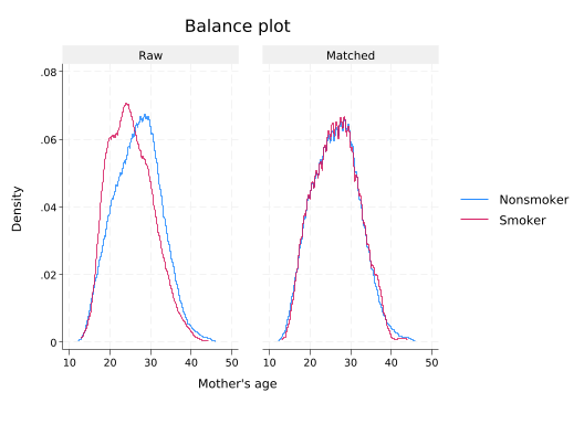
tebalance density medu(refitting the model using the generate() option)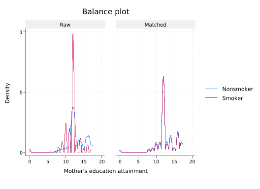
tebalance density fedu(refitting the model using the generate() option)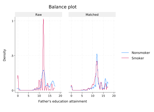
Note how even though fedu was not part of the treatment model, it still looks much more similar after matching.
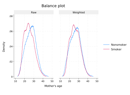
An alternative to propensity score matching is inverse probability weighting. It also relies on using probability of treatment as measure of similarity, but not for matching purposes. Instead, it notes that a treated observation that had a low probability of being treated looks more like a control observation, and a control observation with a low probability of being a control looks more like a treated observation. Giving these low probability observations a higher weight makes the control and treated groups more similar.
teffects ipw (bweight) (mbsmoke medu prenatal1 alcohol mage)
Iteration 0:  EE criterion =  6.651e-21
Iteration 1:  EE criterion =  1.119e-26

Treatment-effects estimation                    Number of obs     =      4,642
Estimator      : inverse-probability weights
Outcome model  : weighted mean
Treatment model: logit
------------------------------------------------------------------------------
             |               Robust
     bweight | Coefficient  std. err.      z    P>|z|     [95% conf. interval]
-------------+----------------------------------------------------------------
ATE          |
     mbsmoke |
    (Smoker  |
         vs  |
 Nonsmoker)  |  -251.7492   23.60685   -10.66   0.000    -298.0178   -205.4806
-------------+----------------------------------------------------------------
POmean       |
     mbsmoke |
  Nonsmoker  |   3404.668   9.511687   357.95   0.000     3386.026    3423.311
------------------------------------------------------------------------------
You can use the same kinds of diagnostics.
teoverlap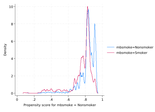
tebalance summarize
Covariate balance summary

                         Raw     Weighted
-----------------------------------------
Number of obs =        4,642      4,642.0
Treated obs   =          864      2,264.4
Control obs   =        3,778      2,377.6
-----------------------------------------

-----------------------------------------------------------------
                |Standardized differences          Variance ratio
                |        Raw    Weighted           Raw   Weighted
----------------+------------------------------------------------
           medu |  -.5474357   -.1355087      .7315846   .4691748
      prenatal1 |  -.3242695   -.0312717      1.496155   1.046148
        alcohol |   .3222725    .0052378      4.509207   1.028204
           mage |   -.300179   -.0633314      .8818025   .8609345
-----------------------------------------------------------------
tebalance density mage