clear all
use https://sscc.wisc.edu/~rdimond/pa871/salaries.dta2 Regression
An introduction to regression usually starts with drawing lines on a scatter plot, which is great as a motivator for the technique but makes something as simple as an indicator variable a strange special case. So we’re going to start with the simplest model possible.
Start a do file. We’ll play fast and loose and not keep a log, but do start with a clear all so it’s reproducible. Then load the example data set salaries (copy and paste highly recommended).
2.1 Constant-Only Model
What we have here is fictional data from 100,000 employees at a firm. Now suppose you were given this data, and then asked to guess the salary of an employee–but you were told absolutely nothing about them. Of course you aren’t expected to get their salary right; the goal is to be off by as little as possible.
The median or the mean value seem like good guesses. If we stipulate that the goal is to minimize the difference between your guess and the actual salary squared, then it’s possible to prove that the mean is the best guess. Find the mean with the sum command (salary is measured in thousands of dollars).
sum salary
    Variable |        Obs        Mean    Std. dev.       Min        Max
-------------+---------------------------------------------------------
      salary |    100,000    67.65335    25.70563   21.11117   181.7357
If you run a regression model for salary with no predictors, i.e. you don’t tell the model anything about the employees other than their salaries, it will make the exact same guess.
reg salary
      Source |       SS           df       MS      Number of obs   =   100,000
-------------+----------------------------------   F(0, 99999)     =      0.00
       Model |           0         0           .   Prob > F        =         .
    Residual |  66077289.3    99,999    660.7795   R-squared       =    0.0000
-------------+----------------------------------   Adj R-squared   =    0.0000
       Total |  66077289.3    99,999    660.7795   Root MSE        =    25.706

------------------------------------------------------------------------------
      salary | Coefficient  Std. err.      t    P>|t|     [95% conf. interval]
-------------+----------------------------------------------------------------
       _cons |   67.65335   .0812883   832.26   0.000     67.49402    67.81267
------------------------------------------------------------------------------
The constant in this regression model is just the mean of salary, and since there are no other predictors that’s the predicted value of salary for all observations.
2.2 Indicator Variables
The firm has carried out a training program (in fact they’ve hired you to evaluate whether the program worked). Now suppose you’re told whether the employee completed the training program or not and asked to guess their salary. Assuming the training program had some impact on salary, a good guess for someone who completed the program would be the mean salary of all employees who completed the program, while a good guess for someone who did not complete the program would be the mean salary of all the employees who did not.
bysort train: sum salary
-------------------------------------------------------------------------------
-> train = Untrained

    Variable |        Obs        Mean    Std. dev.       Min        Max
-------------+---------------------------------------------------------
      salary |     66,204    71.11991    27.31844   21.11117   181.7357

-------------------------------------------------------------------------------
-> train = Trained

    Variable |        Obs        Mean    Std. dev.       Min        Max
-------------+---------------------------------------------------------
      salary |     33,796    60.86258    20.58193   25.54803    181.204
An alternative way to get the same numbers:
tab train, sum(salary)
            |          Summary of salary
      train |        Mean   Std. dev.       Freq.
------------+------------------------------------
  Untrained |   71.119912   27.318445      66,204
    Trained |   60.862584    20.58193      33,796
------------+------------------------------------
      Total |   67.653345   25.705632     100,000
(Things do not look good for this training program, but don’t pass judgment just yet.)
A regression that adds train as a predictor (more precisely, i.train since train is an indicator variable) will make the same guesses, but describe them in a different way.
reg salary i.train
      Source |       SS           df       MS      Number of obs   =   100,000
-------------+----------------------------------   F(1, 99998)     =   3694.12
       Model |  2354062.69         1  2354062.69   Prob > F        =    0.0000
    Residual |  63723226.6    99,998  637.245011   R-squared       =    0.0356
-------------+----------------------------------   Adj R-squared   =    0.0356
       Total |  66077289.3    99,999    660.7795   Root MSE        =    25.244

------------------------------------------------------------------------------
      salary | Coefficient  Std. err.      t    P>|t|     [95% conf. interval]
-------------+----------------------------------------------------------------
       train |
    Trained  |  -10.25733   .1687635   -60.78   0.000     -10.5881   -9.926554
       _cons |   71.11991   .0981095   724.90   0.000     70.92762    71.31221
------------------------------------------------------------------------------
The constant is the mean of salary for untrained. The coefficent Trained is the difference between the two groups: 71.11991 - 10.25733 = 60.86258, the mean salary of the employees who completed the training. This allows you to test the hypothesis that the mean of salary is different for the two groups just by looking at the p-value on Trained. In fact, it’s equivalent to running a t-test.
ttest salary, by(train)
Two-sample t test with equal variances
------------------------------------------------------------------------------
   Group |     Obs        Mean    Std. err.   Std. dev.   [95% conf. interval]
---------+--------------------------------------------------------------------
Untraine |  66,204    71.11991    .1061729    27.31844    70.91181    71.32801
 Trained |  33,796    60.86258    .1119576    20.58193    60.64314    61.08202
---------+--------------------------------------------------------------------
Combined | 100,000    67.65335    .0812883    25.70563    67.49402    67.81267
---------+--------------------------------------------------------------------
    diff |            10.25733    .1687635                9.926554     10.5881
------------------------------------------------------------------------------
    diff = mean(Untraine) - mean(Trained)                         t =  60.7793
H0: diff = 0                                     Degrees of freedom =    99998

    Ha: diff < 0                 Ha: diff != 0                 Ha: diff > 0
 Pr(T < t) = 1.0000         Pr(|T| > |t|) = 0.0000          Pr(T > t) = 0.0000
In this regression, the untrained are the reference group. The coefficient on Trained then tells you the difference between the trained group and the reference group (untrained).
But what if you want to know the predicted value of salary for the trained group based on the regression model? Do you have to do (gasp) math? Of course not. The margins command will do it for you:
margins train
Adjusted predictions                                   Number of obs = 100,000
Model VCE: OLS

Expression: Linear prediction, predict()

------------------------------------------------------------------------------
             |            Delta-method
             |     Margin   std. err.      t    P>|t|     [95% conf. interval]
-------------+----------------------------------------------------------------
       train |
  Untrained  |   71.11991   .0981095   724.90   0.000     70.92762    71.31221
    Trained  |   60.86258   .1373158   443.23   0.000     60.59345    61.13172
------------------------------------------------------------------------------
Those numbers are equal to the mean salaries of the two groups. But that’s not actually what margins does. Asked to calculate margins for train, which it knows is an indicator variable because you put i.train in your regression, it first sets everyone’s value of train to 0, calculates everyone’s predicted salary, and reports the mean. Then it sets everyone’s value of train to 0 and repeats the process. You’ll see why that’s important soon.
You can also ask margins to calculate the difference between the two groups with the dydx() option.
margins, dydx(train)
Conditional marginal effects                           Number of obs = 100,000
Model VCE: OLS

Expression: Linear prediction, predict()
dy/dx wrt:  1.train

------------------------------------------------------------------------------
             |            Delta-method
             |      dy/dx   std. err.      t    P>|t|     [95% conf. interval]
-------------+----------------------------------------------------------------
       train |
    Trained  |  -10.25733   .1687635   -60.78   0.000     -10.5881   -9.926554
------------------------------------------------------------------------------
Note: dy/dx for factor levels is the discrete change from the base level.
Since this is a linear model, the result is just the coefficient on Trained. But in more complicated models this can be very useful.
2.3 Categorical Variables
Now suppose that instead of train you know edu, the employee’s education level. It’s a categorical variable with 3 categories, or levels. Again, a good guess would be the mean salary for everyone with that level of education.
tab edu, sum(salary)
            |          Summary of salary
        edu |        Mean   Std. dev.       Freq.
------------+------------------------------------
  High Scho |    43.56295    9.869016      32,972
   Bachelor |   71.086272   9.2926206      57,481
   Advanced |   130.18403   8.9240392       9,547
------------+------------------------------------
      Total |   67.653345   25.705632     100,000
And that’s what a regression will do too, but again it reports it in terms of a reference level and then differences from it.
reg salary i.edu
      Source |       SS           df       MS      Number of obs   =   100,000
-------------+----------------------------------   F(2, 99997)     >  99999.00
       Model |  57142209.4         2  28571104.7   Prob > F        =    0.0000
    Residual |   8935079.9    99,997  89.3534796   R-squared       =    0.8648
-------------+----------------------------------   Adj R-squared   =    0.8648
       Total |  66077289.3    99,999    660.7795   Root MSE        =    9.4527

------------------------------------------------------------------------------
      salary | Coefficient  Std. err.      t    P>|t|     [95% conf. interval]
-------------+----------------------------------------------------------------
         edu |
   Bachelor  |   27.52332   .0653029   421.47   0.000     27.39533    27.65132
   Advanced  |   86.62108   .1098604   788.47   0.000     86.40575     86.8364
             |
       _cons |   43.56295   .0520575   836.82   0.000     43.46092    43.66498
------------------------------------------------------------------------------
By default, Stata will use the lowest value as the reference. You can change that if you want to:
reg salary ib2.edu
      Source |       SS           df       MS      Number of obs   =   100,000
-------------+----------------------------------   F(2, 99997)     >  99999.00
       Model |  57142209.4         2  28571104.7   Prob > F        =    0.0000
    Residual |   8935079.9    99,997  89.3534796   R-squared       =    0.8648
-------------+----------------------------------   Adj R-squared   =    0.8648
       Total |  66077289.3    99,999    660.7795   Root MSE        =    9.4527

------------------------------------------------------------------------------
      salary | Coefficient  Std. err.      t    P>|t|     [95% conf. interval]
-------------+----------------------------------------------------------------
         edu |
High School  |  -86.62108   .1098604  -788.47   0.000     -86.8364   -86.40575
   Bachelor  |  -59.09775   .1044692  -565.70   0.000    -59.30251   -58.89299
             |
       _cons |    130.184   .0967436  1345.66   0.000     129.9944    130.3736
------------------------------------------------------------------------------
Note how the effect of Advanced compared to the base level High School is just the negative of the effect of High School compared to the base level Advanced. These are fundamentally the same model (they give the same predicted values), just described differently.
margins works the same way as with an indicator, just with more levels to report.
margins edu
Adjusted predictions                                   Number of obs = 100,000
Model VCE: OLS

Expression: Linear prediction, predict()

------------------------------------------------------------------------------
             |            Delta-method
             |     Margin   std. err.      t    P>|t|     [95% conf. interval]
-------------+----------------------------------------------------------------
         edu |
High School  |   43.56295   .0520575   836.82   0.000     43.46092    43.66498
   Bachelor  |   71.08627    .039427  1802.99   0.000       71.009    71.16355
   Advanced  |    130.184   .0967436  1345.66   0.000     129.9944    130.3736
------------------------------------------------------------------------------
margins, dydx(edu)
Conditional marginal effects                           Number of obs = 100,000
Model VCE: OLS

Expression: Linear prediction, predict()
dy/dx wrt:  0.edu 1.edu

------------------------------------------------------------------------------
             |            Delta-method
             |      dy/dx   std. err.      t    P>|t|     [95% conf. interval]
-------------+----------------------------------------------------------------
         edu |
High School  |  -86.62108   .1098604  -788.47   0.000     -86.8364   -86.40575
   Bachelor  |  -59.09775   .1044692  -565.70   0.000    -59.30251   -58.89299
------------------------------------------------------------------------------
Note: dy/dx for factor levels is the discrete change from the base level.
2.4 Categorical Interactions
Now suppose you know both train and edu so your guess will be the mean value for people with the same level of both variables.
tab edu train, sum(salary)
           Means, Standard Deviations and Frequencies of salary

           |        train
       edu | Untrained    Trained |     Total
-----------+----------------------+----------
 High Scho | 41.589563  45.510414 |  43.56295
           | 9.7972257   9.547799 |  9.869016
           |     16377      16595 |     32972
-----------+----------------------+----------
  Bachelor |  70.86273  71.665069 | 71.086272
           | 9.3972106  8.9906781 | 9.2926206
           |     41466      16015 |     57481
-----------+----------------------+----------
  Advanced | 130.23758  129.80647 | 130.18403
           | 8.9427914  8.7851637 | 8.9240392
           |      8361       1186 |      9547
-----------+----------------------+----------
     Total | 71.119912  60.862584 | 67.653345
           | 27.318445   20.58193 | 25.705632
           |     66204      33796 |    100000
Or if you’d prefer a simpler table, use table instead of tabulate.
table (edu) (train), stat(mean salary) nototal
-------------------------------------
              |          train
              |  Untrained    Trained
--------------+----------------------
edu           |
  High School |   41.58956   45.51041
  Bachelor    |   70.86273   71.66507
  Advanced    |   130.2376   129.8065
-------------------------------------
Note how the difference between the trained and untrained is different for each education level. To allow this in a regression model, we need to include an interaction between train and edu in the predictors. Putting ## between two variables means to include both the variables alone (their main effect) and the interaction between them. # between two variables refers to just the interaction. Variables in interactions are assumed to be factor variables, so we don’t need to put i. before them.
reg salary train##edu
      Source |       SS           df       MS      Number of obs   =   100,000
-------------+----------------------------------   F(5, 99994)     >  99999.00
       Model |  57276554.4         5  11455310.9   Prob > F        =    0.0000
    Residual |  8800734.89    99,994  88.0126297   R-squared       =    0.8668
-------------+----------------------------------   Adj R-squared   =    0.8668
       Total |  66077289.3    99,999    660.7795   Root MSE        =    9.3815

------------------------------------------------------------------------------
      salary | Coefficient  Std. err.      t    P>|t|     [95% conf. interval]
-------------+----------------------------------------------------------------
       train |
    Trained  |   3.920852   .1033331    37.94   0.000      3.71832    4.123383
             |
         edu |
   Bachelor  |   29.27317   .0865834   338.09   0.000     29.10346    29.44287
   Advanced  |   88.64802   .1260981   703.01   0.000     88.40087    88.89517
             |
   train#edu |
    Trained #|
   Bachelor  |  -3.118512   .1352623   -23.06   0.000    -3.383625     -2.8534
    Trained #|
   Advanced  |  -4.351964   .3088915   -14.09   0.000    -4.957387    -3.74654
             |
       _cons |   41.58956   .0733087   567.32   0.000     41.44588    41.73325
------------------------------------------------------------------------------
Now Trained is the effect of training for the base category of edu, High School. Meanwhile Bachelor and Advanced is the effect of edu for the base category of train, which is Untrained. The interaction terms Trained#Bachelor and Trained#Advanced are the additional effect to be added if someone is both trained and has that level of education.
This looks confusing, but if you have margins add it all up you’ll see it’s still just the means.
margins edu#train
Adjusted predictions                                   Number of obs = 100,000
Model VCE: OLS

Expression: Linear prediction, predict()

------------------------------------------------------------------------------
             |            Delta-method
             |     Margin   std. err.      t    P>|t|     [95% conf. interval]
-------------+----------------------------------------------------------------
   edu#train |
High School #|
  Untrained  |   41.58956   .0733087   567.32   0.000     41.44588    41.73325
High School #|
    Trained  |   45.51041   .0728256   624.92   0.000     45.36768    45.65315
   Bachelor #|
  Untrained  |   70.86273   .0460709  1538.12   0.000     70.77243    70.95303
   Bachelor #|
    Trained  |   71.66507   .0741326   966.72   0.000     71.51977    71.81037
   Advanced #|
  Untrained  |   130.2376   .1025991  1269.38   0.000     130.0365    130.4387
   Advanced #|
    Trained  |   129.8065   .2724145   476.50   0.000     129.2725    130.3404
------------------------------------------------------------------------------
marginsplot automatically makes a data visualization out of these numbers.
marginsplot
Variables that uniquely identify margins: edu train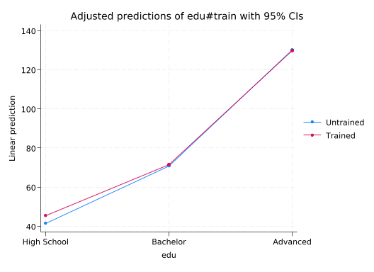
We can also ask margins to add up the total effect of train at each level of edu.
margins edu, dydx(train)
Conditional marginal effects                           Number of obs = 100,000
Model VCE: OLS

Expression: Linear prediction, predict()
dy/dx wrt:  1.train

------------------------------------------------------------------------------
             |            Delta-method
             |      dy/dx   std. err.      t    P>|t|     [95% conf. interval]
-------------+----------------------------------------------------------------
0.train      |  (base outcome)
-------------+----------------------------------------------------------------
1.train      |
         edu |
High School  |   3.920852   .1033331    37.94   0.000      3.71832    4.123383
   Bachelor  |   .8023392   .0872821     9.19   0.000     .6312674     .973411
   Advanced  |  -.4311121   .2910948    -1.48   0.139    -1.001654    .1394302
------------------------------------------------------------------------------
Note: dy/dx for factor levels is the discrete change from the base level.
2.5 Categorical Variables Without Interactions
It’s uncommon to be able to reliably estimate interactions like that–most data sets have fewer than the 100,000 observations we’ve been using. So we commonly assume variables have the same effect for all observations.
reg salary i.edu i.train
      Source |       SS           df       MS      Number of obs   =   100,000
-------------+----------------------------------   F(3, 99996)     >  99999.00
       Model |  57223444.8         3  19074481.6   Prob > F        =    0.0000
    Residual |  8853844.46    99,996  88.5419863   R-squared       =    0.8660
-------------+----------------------------------   Adj R-squared   =    0.8660
       Total |  66077289.3    99,999    660.7795   Root MSE        =    9.4097

------------------------------------------------------------------------------
      salary | Coefficient  Std. err.      t    P>|t|     [95% conf. interval]
-------------+----------------------------------------------------------------
         edu |
   Bachelor  |     27.967   .0666356   419.70   0.000      27.8364    28.09761
   Advanced  |   87.36961   .1121178   779.27   0.000     87.14986    87.58936
             |
       train |
    Trained  |   1.974619   .0651906    30.29   0.000     1.846846    2.102392
       _cons |   42.56911   .0613345   694.05   0.000      42.4489    42.68933
------------------------------------------------------------------------------
The mean predicted salaries no longer line up exactly with the observed means.
table (edu) (train), stat(mean salary) nototal
margins edu#train
-------------------------------------
              |          train
              |  Untrained    Trained
--------------+----------------------
edu           |
  High School |   41.58956   45.51041
  Bachelor    |   70.86273   71.66507
  Advanced    |   130.2376   129.8065
-------------------------------------

Adjusted predictions                                   Number of obs = 100,000
Model VCE: OLS

Expression: Linear prediction, predict()

------------------------------------------------------------------------------
             |            Delta-method
             |     Margin   std. err.      t    P>|t|     [95% conf. interval]
-------------+----------------------------------------------------------------
   edu#train |
High School #|
  Untrained  |   42.56911   .0613345   694.05   0.000      42.4489    42.68933
High School #|
    Trained  |   44.54373    .061105   728.97   0.000     44.42397     44.6635
   Bachelor #|
  Untrained  |   70.53612   .0432466  1631.02   0.000     70.45135    70.62088
   Bachelor #|
    Trained  |   72.51074   .0612533  1183.79   0.000     72.39068    72.63079
   Advanced #|
  Untrained  |   129.9387   .0966432  1344.52   0.000     129.7493    130.1281
   Advanced #|
    Trained  |   131.9133   .1119546  1178.27   0.000     131.6939    132.1328
------------------------------------------------------------------------------
marginsplot makes it easy to see the difference between this model and the previous one.
marginsplot
Variables that uniquely identify margins: edu train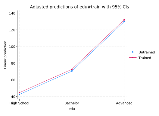
2.5.1 Continuous Predictors
Now suppose we know the tenure (years worked at the company, not “has tenure” like in academia) of each employee, a continuous variable. Now we’ve finally gotten to drawing lines on scatterplots.
scatter salary tenure, msize(tiny) || lfit salary tenure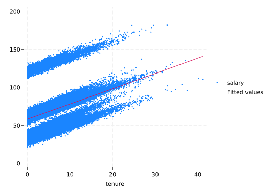
regress will estimate the slope of that line.
regress salary tenure
      Source |       SS           df       MS      Number of obs   =   100,000
-------------+----------------------------------   F(1, 99998)     =  12321.47
       Model |   7248691.6         1   7248691.6   Prob > F        =    0.0000
    Residual |  58828597.7    99,998  588.297743   R-squared       =    0.1097
-------------+----------------------------------   Adj R-squared   =    0.1097
       Total |  66077289.3    99,999    660.7795   Root MSE        =    24.255

------------------------------------------------------------------------------
      salary | Coefficient  Std. err.      t    P>|t|     [95% conf. interval]
-------------+----------------------------------------------------------------
      tenure |   2.009571   .0181039   111.00   0.000     1.974088    2.045055
       _cons |   57.62375     .11852   486.19   0.000     57.39145    57.85605
------------------------------------------------------------------------------
This means the predicted starting salary is \$57.6k and salaries increase by \$2k for every year of tenure.
But we know edu makes a big difference, so add it to the model.
reg salary tenure i.edu
      Source |       SS           df       MS      Number of obs   =   100,000
-------------+----------------------------------   F(3, 99996)     >  99999.00
       Model |  64476272.6         3  21492090.9   Prob > F        =    0.0000
    Residual |  1601016.69    99,996  16.0108073   R-squared       =    0.9758
-------------+----------------------------------   Adj R-squared   =    0.9758
       Total |  66077289.3    99,999    660.7795   Root MSE        =    4.0014

------------------------------------------------------------------------------
      salary | Coefficient  Std. err.      t    P>|t|     [95% conf. interval]
-------------+----------------------------------------------------------------
      tenure |   2.021376   .0029866   676.81   0.000     2.015522     2.02723
             |
         edu |
   Bachelor  |    27.5267   .0276429   995.80   0.000     27.47252    27.58088
   Advanced  |   86.69164   .0465043  1864.16   0.000     86.60049    86.78278
             |
       _cons |   33.46576   .0266113  1257.58   0.000      33.4136    33.51792
------------------------------------------------------------------------------
Salaries still go up by about \$2k/year, but the expected starting salary depends on education: \$33.5k for high school, plus \$27.5k for a Bachelor’s, or \$86.7k for an advanced degree. margins and marginsplot can be really useful here, but since tenure is continuous we need the at() option to specify the values we’re interested in.
margins edu, at(tenure=(0(5)20))
marginsplot, addplot(scatter salary tenure, below)
Adjusted predictions                                   Number of obs = 100,000
Model VCE: OLS

Expression: Linear prediction, predict()
1._at: tenure =  0
2._at: tenure =  5
3._at: tenure = 10
4._at: tenure = 15
5._at: tenure = 20

------------------------------------------------------------------------------
             |            Delta-method
             |     Margin   std. err.      t    P>|t|     [95% conf. interval]
-------------+----------------------------------------------------------------
     _at#edu |
          1 #|
High School  |   33.46576   .0266113  1257.58   0.000      33.4136    33.51792
 1#Bachelor  |   60.99246   .0223822  2725.04   0.000     60.94859    61.03633
 1#Advanced  |   120.1574   .0435491  2759.13   0.000      120.072    120.2428
          2 #|
High School  |   43.57264   .0220361  1977.33   0.000     43.52945    43.61583
 2#Bachelor  |   71.09934   .0166896  4260.11   0.000     71.06663    71.13205
 2#Advanced  |   130.2643    .040952  3180.90   0.000      130.184    130.3445
          3 #|
High School  |   53.67952   .0266273  2015.96   0.000     53.62733    53.73171
 3#Bachelor  |   81.20622    .022408  3623.99   0.000      81.1623    81.25014
 3#Advanced  |   140.3712   .0436303  3217.28   0.000     140.2856    140.4567
          4 #|
High School  |    63.7864   .0371273  1718.04   0.000     63.71363    63.85917
 4#Bachelor  |    91.3131     .03423  2667.64   0.000     91.24601    91.38019
 4#Advanced  |    150.478   .0507557  2964.75   0.000     150.3786    150.5775
          5 #|
High School  |   73.89328   .0499386  1479.68   0.000      73.7954    73.99116
 5#Bachelor  |     101.42   .0478253  2120.63   0.000     101.3262    101.5137
 5#Advanced  |   160.5849   .0607839  2641.90   0.000     160.4658    160.7041
------------------------------------------------------------------------------

Variables that uniquely identify margins: tenure edu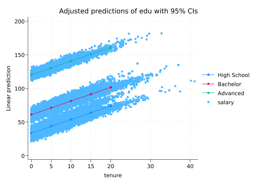
2.6 Interactions With Continuous Variables
Now let’s look at how training affects the relationship between tenure and salary.
scatter salary tenure, colorvar(train) colordisc msize(tiny) coloruseplegend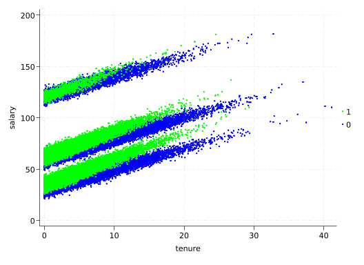
The slope of the tenure line is different for trained employees than for untrained employees! This again calls for an interaction in the regression model. Remember that Stata assumes variables in interactions are factor variables, so we need to put c. in front of tenure to specify that it is continuous.
reg salary train##c.tenure
      Source |       SS           df       MS      Number of obs   =   100,000
-------------+----------------------------------   F(3, 99996)     =   4980.77
       Model |  8590233.06         3  2863411.02   Prob > F        =    0.0000
    Residual |  57487056.2    99,996  574.893558   R-squared       =    0.1300
-------------+----------------------------------   Adj R-squared   =    0.1300
       Total |  66077289.3    99,999    660.7795   Root MSE        =    23.977

------------------------------------------------------------------------------
      salary | Coefficient  Std. err.      t    P>|t|     [95% conf. interval]
-------------+----------------------------------------------------------------
       train |
    Trained  |  -9.979142   .2475621   -40.31   0.000    -10.46436   -9.493924
      tenure |   1.743132   .0207497    84.01   0.000     1.702463    1.783801
             |
       train#|
    c.tenure |
    Trained  |   .5530884   .0426809    12.96   0.000     .4694344    .6367424
             |
       _cons |   61.57144   .1469786   418.91   0.000     61.28336    61.85952
------------------------------------------------------------------------------
This suggests Trained people have lower starting salaries by about \$10k, but while salaries for Untrained people go up by \$1.7k/year of tenure, salaries for trained people go up by \$2.3k/year of tenure (1.743132 + .5530884). margins will make it easy to see the overall effect.
margins train, at(tenure=(0(5)20))
marginsplot
Adjusted predictions                                   Number of obs = 100,000
Model VCE: OLS

Expression: Linear prediction, predict()
1._at: tenure =  0
2._at: tenure =  5
3._at: tenure = 10
4._at: tenure = 15
5._at: tenure = 20

------------------------------------------------------------------------------
             |            Delta-method
             |     Margin   std. err.      t    P>|t|     [95% conf. interval]
-------------+----------------------------------------------------------------
   _at#train |
1#Untrained  |   61.57144   .1469786   418.91   0.000     61.28336    61.85952
  1#Trained  |    51.5923   .1992091   258.99   0.000     51.20185    51.98274
2#Untrained  |    70.2871    .093712   750.03   0.000     70.10342    70.47077
  2#Trained  |    63.0734   .1352784   466.25   0.000     62.80825    63.33854
3#Untrained  |   79.00276   .1322446   597.40   0.000     78.74356    79.26195
  3#Trained  |    74.5545   .2578209   289.17   0.000     74.04917    75.05982
4#Untrained  |   87.71842   .2184555   401.54   0.000     87.29025    88.14659
  4#Trained  |    86.0356   .4291834   200.46   0.000     85.19441    86.87679
5#Untrained  |   96.43407   .3154115   305.74   0.000     95.81587    97.05228
  5#Trained  |    97.5167    .609492   160.00   0.000      96.3221     98.7113
------------------------------------------------------------------------------

Variables that uniquely identify margins: tenure train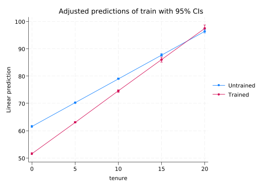
2.7 The Complete Model
But why would a training program reduce starting salaries? Well, let’s look at who gets trained.
tab edu train, row
+----------------+
| Key            |
|----------------|
|   frequency    |
| row percentage |
+----------------+

            |         train
        edu | Untrained    Trained |     Total
------------+----------------------+----------
High School |    16,377     16,595 |    32,972
            |     49.67      50.33 |    100.00
------------+----------------------+----------
   Bachelor |    41,466     16,015 |    57,481
            |     72.14      27.86 |    100.00
------------+----------------------+----------
   Advanced |     8,361      1,186 |     9,547
            |     87.58      12.42 |    100.00
------------+----------------------+----------
      Total |    66,204     33,796 |   100,000
            |     66.20      33.80 |    100.00
About half of employees with a high school education get trained, but only 28% of those with a Bachelor’s degree and 12% of those with an advanced degree. Given the very strong relationship between edu and salary, trying to estimate the effect of train on salary without controlling for edu is going to be a disaster. We also saw evidence that the effect of train depends on edu, and the effect of tenure depends on train, so we’ll include both interactions.
regress salary train##(c.tenure i.edu)
      Source |       SS           df       MS      Number of obs   =   100,000
-------------+----------------------------------   F(7, 99992)     >  99999.00
       Model |  65176547.2         7  9310935.32   Prob > F        =    0.0000
    Residual |  900742.041    99,992  9.00814106   R-squared       =    0.9864
-------------+----------------------------------   Adj R-squared   =    0.9864
       Total |  66077289.3    99,999    660.7795   Root MSE        =    3.0014

------------------------------------------------------------------------------
      salary | Coefficient  Std. err.      t    P>|t|     [95% conf. interval]
-------------+----------------------------------------------------------------
       train |
    Trained  |   4.930425   .0413136   119.34   0.000     4.849451    5.011399
      tenure |   1.996295   .0026001   767.76   0.000     1.991199    2.001392
             |
         edu |
   Bachelor  |   29.99815   .0277161  1082.34   0.000     29.94383    30.05247
   Advanced  |   90.00605   .0403804  2228.95   0.000      89.9269     90.0852
             |
       train#|
    c.tenure |
    Trained  |   .5101078   .0053488    95.37   0.000     .4996242    .5205914
             |
   train#edu |
    Trained #|
   Bachelor  |   -2.98867   .0433131   -69.00   0.000    -3.073563   -2.903776
    Trained #|
   Advanced  |  -4.930725   .0988479   -49.88   0.000    -5.124465   -4.736984
             |
       _cons |   30.02873   .0278709  1077.42   0.000      29.9741    30.08335
------------------------------------------------------------------------------
With an R-squared of .986 and coefficients that are extremely close to round numbers, you can tell this is 1) made-up data and 2) a model that matches the data-generating process.
marginsplot can make this easy to understand (I’ll omit the margins output for convenience).
quietly margins edu#train, at(tenure=(0(5)20))
marginsplot
Variables that uniquely identify margins: tenure edu train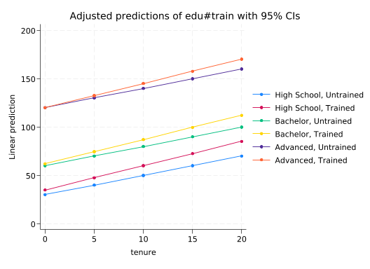
And the effect of train?
quietly margins edu, dydx(train) at(tenure=(0(5)20))
marginsplot
Variables that uniquely identify margins: tenure edu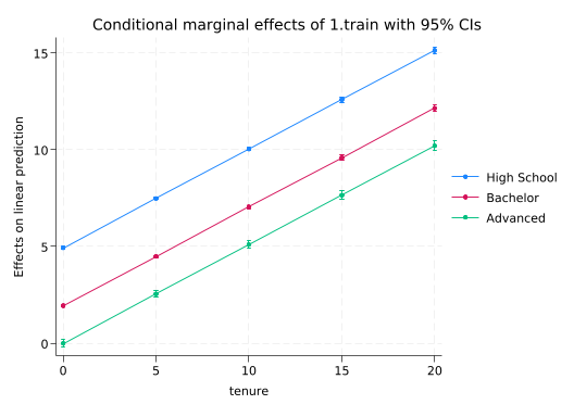
For those with advanced degrees, train only has an effect via tenure. But for those with less education, it has both an effect on its own and the effect through tenure. Note that we did not include a three-way interaction between train, edu, and tenure so the increase in the effect of tenure associated with train is the same for all levels of edu.
2.8 Diagnostics
Before we trust this model we should do at least some regression diagnostics. But the right diagnostics.
salary is not remotely normal–like most salary distributions, it is right-skewed.
sum salary, detail
hist salary
                           salary
-------------------------------------------------------------
      Percentiles      Smallest
 1%      29.5404       21.11117
 5%     34.22136       21.49281
10%      37.6162       21.52696       Obs             100,000
25%     49.12166       22.31187       Sum of wgt.     100,000

50%     65.60289                      Mean           67.65335
                        Largest       Std. dev.      25.70563
75%     75.53474       178.1305
90%     101.6421        181.204       Variance       660.7795
95%     127.9607       181.3195       Skewness        1.13581
99%     141.6542       181.7357       Kurtosis       4.343584
(bin=50, start=21.111168, width=3.2124898)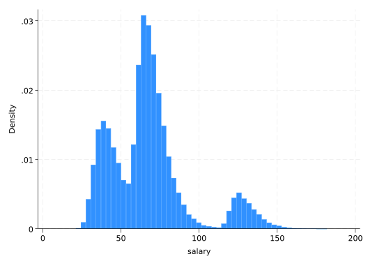
Is that a problem? Should we be using a log transform to make it more normal? No. OLS regression does not require that the outcome variable be normally distributed; it requires that the residuals be normally distributed. You can calculate the residuals with the predict command and residual option.
predict residuals, residualNow look at their distribution.
hist residuals(bin=50, start=-12.927955, width=.50254992)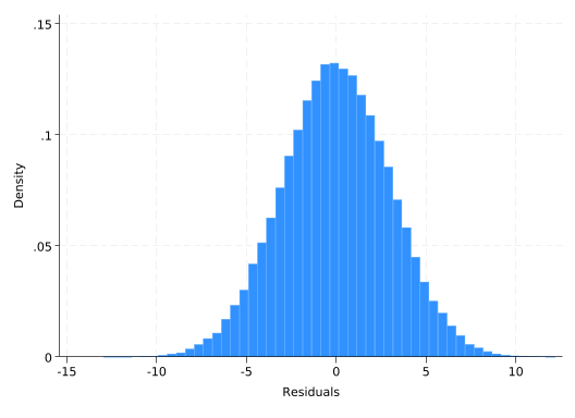
qnorm residuals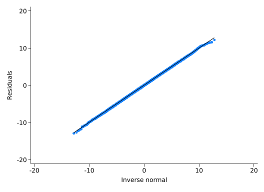
That’s more normal than you’ll ever see with real data. The model successfully explained all the non-normal components of salary.
A right-skewed distribution can suggest your data-generating process is multiplicative: if you add a bunch of random numbers the result will be normal, but if you multiply a bunch of random numbers the result will be log-normal, which is right-skewed. Taking the log will make a multiplicative process additive and a good candidate for a linear model. But check the residuals themselves before you assume such a process.
Residuals should be independent of both the predicted (or fitted) values and the continuous predictors. If you see a relationship between them, then that suggests there’s something wrong or missing in your model. rvfplot (residuals vs fitted values) will get the first, scatter will get you the rest.
rvfplot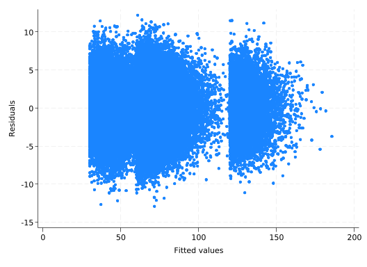
The residuals should always be centered around zero. Don’t be fooled by the fact that areas with lots of points will have more outliers.
scatter res tenure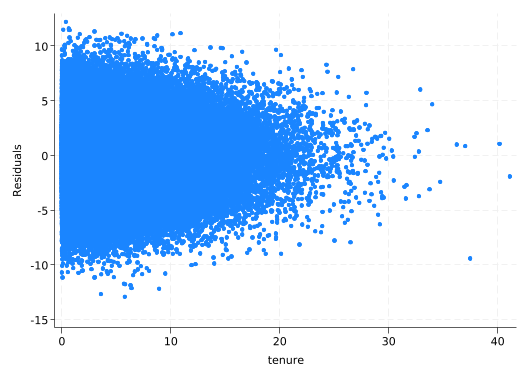
What would it look like if we did a log transform?
gen log_salary = ln(salary)reg log_salary train##(c.tenure i.edu)
quietly margins edu#train, at(tenure=(0(5)20)) expression(exp(predict(xb)))
marginsplot
      Source |       SS           df       MS      Number of obs   =   100,000
-------------+----------------------------------   F(7, 99992)     >  99999.00
       Model |  12801.2091         7  1828.74416   Prob > F        =    0.0000
    Residual |  473.811329    99,992  .004738492   R-squared       =    0.9643
-------------+----------------------------------   Adj R-squared   =    0.9643
       Total |  13275.0205    99,999  .132751532   Root MSE        =    .06884

------------------------------------------------------------------------------
  log_salary | Coefficient  Std. err.      t    P>|t|     [95% conf. interval]
-------------+----------------------------------------------------------------
       train |
    Trained  |   .0934263   .0009475    98.60   0.000     .0915692    .0952835
      tenure |    .029955   .0000596   502.31   0.000     .0298381    .0300719
             |
         edu |
   Bachelor  |   .5610196   .0006357   882.56   0.000     .5597737    .5622655
   Advanced  |   1.185096   .0009261  1279.62   0.000     1.183281    1.186911
             |
       train#|
    c.tenure |
    Trained  |   .0117355   .0001227    95.66   0.000      .011495    .0119759
             |
   train#edu |
    Trained #|
   Bachelor  |  -.0799929   .0009934   -80.52   0.000    -.0819399   -.0780459
    Trained #|
   Advanced  |  -.1061102   .0022671   -46.80   0.000    -.1105536   -.1016667
             |
       _cons |   3.528906   .0006392  5520.61   0.000     3.527653    3.530158
------------------------------------------------------------------------------

Variables that uniquely identify margins: tenure edu train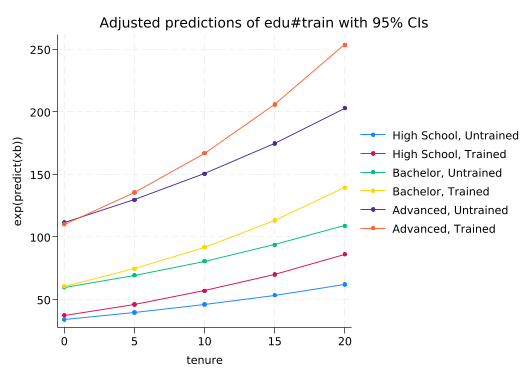
Assuming a log-linear form introduced a curve into our model even though there’s no curve in the data. The model will fit it as best it can, but the curved line will be too high at the right and left ends and too low in the middle. Thus the residuals will be negative on the right and left ends and positive in the middle. You can see that with rvfplot.
rvfplot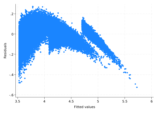
On the other hand, if this data really were log-linear, you’d see the same sort of pattern if you tried to use a linear model. Similar plots could also lead you to include squared terms in your model (a squared term is a second order Taylor series approximation to anything).
2.9 Why You Shouldn’t Use Interactions Lightly
Interactions are hard to estimate–you need some combination of a lot of data, a strong effect, and not much noise. This data set is bigger than you’re likely to work with in the real world, and has a far higher R-squared (i.e. there’s very little noise). The salary2 and train2 variables are more like what you’re likely to actually see. salary2 is a lot less predictable (in the real world we’re lucky to be able to predict 20% of the variation in salaries) and it only has 800 observations. On the other hand, to make things easier train2 is completely random and has a main effect on all education levels so it’s easier to estimate.
Start with a simple model where we assume training has the same effect for everyone.
reg salary2 i.train2 tenure i.edu
      Source |       SS           df       MS      Number of obs   =       800
-------------+----------------------------------   F(4, 795)       =     95.50
       Model |  666617.082         4  166654.271   Prob > F        =    0.0000
    Residual |  1387311.37       795  1745.04575   R-squared       =    0.3246
-------------+----------------------------------   Adj R-squared   =    0.3212
       Total |  2053928.45       799  2570.62385   Root MSE        =    41.774

------------------------------------------------------------------------------
     salary2 | Coefficient  Std. err.      t    P>|t|     [95% conf. interval]
-------------+----------------------------------------------------------------
    1.train2 |   6.986803   3.263948     2.14   0.033      .579828    13.39378
      tenure |   2.290322   .3580977     6.40   0.000     1.587394    2.993251
             |
         edu |
   Bachelor  |   34.40527   3.219203    10.69   0.000     28.08612    40.72441
   Advanced  |   98.55754   5.490826    17.95   0.000     87.77931    109.3358
             |
       _cons |   24.58744   3.220637     7.63   0.000     18.26548     30.9094
------------------------------------------------------------------------------
Great, training has an effect. Now try interacting train2 with everything like we did before.
reg salary2 i.train2##(c.tenure i.edu)
      Source |       SS           df       MS      Number of obs   =       800
-------------+----------------------------------   F(7, 792)       =     54.87
       Model |  670792.162         7  95827.4518   Prob > F        =    0.0000
    Residual |  1383136.29       792  1746.38421   R-squared       =    0.3266
-------------+----------------------------------   Adj R-squared   =    0.3206
       Total |  2053928.45       799  2570.62385   Root MSE        =     41.79

------------------------------------------------------------------------------
     salary2 | Coefficient  Std. err.      t    P>|t|     [95% conf. interval]
-------------+----------------------------------------------------------------
    1.train2 |   5.483388   6.972496     0.79   0.432    -8.203369    19.17014
      tenure |   1.959505   .4406548     4.45   0.000     1.094516    2.824495
             |
         edu |
   Bachelor  |   36.04839   3.783965     9.53   0.000      28.6206    43.47618
   Advanced  |   97.90354   6.464464    15.14   0.000     85.21403     110.593
             |
      train2#|
    c.tenure |
          1  |   .9428405   .7580626     1.24   0.214     -.545209     2.43089
             |
  train2#edu |
 1#Bachelor  |   -5.31276   7.223985    -0.74   0.462    -19.49318    8.867661
 1#Advanced  |   2.261653   12.26855     0.18   0.854    -21.82107    26.34438
             |
       _cons |   25.34002   3.644351     6.95   0.000     18.18629    32.49375
------------------------------------------------------------------------------
Now training has no effect! Since I made the data, I can tell you the effect of train2 does vary with edu and tenure. This is the “right” model in that sense. But it gives you the wrong answer to the question you care about “Does training increase salaries?” The model doesn’t have enough information to precisely estimate all the different ways train2 affects salary2, so they all have large standard errors and are not significantly different from zero. Don’t try to estimate a more complicated model than your data will support, even if you think it’s “right.”
All models are wrong; some models are useful.