set linesize 10010 Exercise Solutions
10.1 Reading in Data
10.1.1 Exercise 1
The details will depend on where you want to put the example files, your username, and the kind of computer you’re using. The example code in the text and repeated here assumes you want to put the example files in a folder on your desktop and your username is bbadger. Modify as needed.
Windows:
cd c:\users\bbadger\desktop
mkdir dws
cd dws
net get dws, from(https://ssc.wisc.edu/sscc/stata/)
MacOS or Linux:
cd /users/bbadger/desktop
mkdir dws
cd dws
net get dws, from(https://ssc.wisc.edu/sscc/stata/)
Exercse 2
clear
use 2000_acs_sample
. clear

. use 2000_acs_sample

.
Exercise 3
After editing to remove the absolute path:
import delimited qualtrics_survey.csv, varnames(1) rowrange(4) colrange(18:21) clear(encoding automatically selected: ISO-8859-1)
(4 vars, 69 obs)Take a look at the values of q1 with tab:
tab q1
                      Q1 |      Freq.     Percent        Cum.
-------------------------+-----------------------------------
                      18 |          7       10.14       10.14
                      19 |         20       28.99       39.13
                      20 |         23       33.33       72.46
                      21 |         10       14.49       86.96
                      22 |          1        1.45       88.41
                      24 |          3        4.35       92.75
                      25 |          1        1.45       94.20
                      27 |          1        1.45       95.65
                      31 |          1        1.45       97.10
                      40 |          1        1.45       98.55
           Between 20-25 |          1        1.45      100.00
-------------------------+-----------------------------------
                   Total |         69      100.00
When asked their age, someone typed in “Between 20-25” instead of a number. This forced Stata to treat the entire column as text. You’ll learn how to deal with problems like this in First Steps With Your Data.
For real work it’s easier to have Qualtrics give you an SPSS data set. Stata can read SPSS data sets, and they’re already structured as data sets so they generally require less work to read.
10.2 First Steps With Your Data
Excercise 1
Be sure to create a new do file for this exercise because it uses a separate dataset. Call it first_steps_exercises.do. Then be sure to switch back to first_steps.do when you go back to following the examples in the book.
The output from label list is quite long, so for the book we’ll comment it out and only list a few specific value labels. You should run the full version and skim the results though!
capture log close
log using first_steps_exercises.log, replace

clear all
use 2000_acs_sample_harm

describe
// label list
label list race_lbl
label list educ_lbl
. capture log close

. log using first_steps_exercises.log, replace
----------------------------------------------------------------------------------------------------
      name:  <unnamed>
       log:  C:\Users\rdimond\dws\first_steps_exercises.log
  log type:  text
 opened on:  11 Jan 2023, 14:33:29

.
. clear all

. use 2000_acs_sample_harm

.
. describe

Contains data from 2000_acs_sample_harm.dta
 Observations:        28,085
    Variables:            18                  19 Mar 2019 13:50
----------------------------------------------------------------------------------------------------
Variable      Storage   Display    Value
    name         type    format    label      Variable label
----------------------------------------------------------------------------------------------------
year            int     %8.0g      year_lbl   Census year
datanum         byte    %8.0g                 Data set number
serial          double  %8.0g                 Household serial number
hhwt            double  %10.2f                Household weight
gq              byte    %43.0g     gq_lbl     Group quarters status
pernum          int     %8.0g                 Person number in sample unit
perwt           double  %10.2f                Person weight
sex             byte    %8.0g      sex_lbl    Sex
age             int     %36.0g     age_lbl    Age
marst           byte    %23.0g     marst_lbl
                                              Marital status
race            byte    %32.0g     race_lbl   Race [general version]
raced           int     %182.0g    raced_lbl
                                              Race [detailed version]
hispan          byte    %12.0g     hispan_lbl
                                              Hispanic origin [general version]
hispand         int     %24.0g     hispand_lbl
                                              Hispanic origin [detailed version]
educ            byte    %25.0g     educ_lbl   Educational attainment [general version]
educd           int     %46.0g     educd_lbl
                                              Educational attainment [detailed version]
inctot          long    %12.0g                Total personal income
ftotinc         long    %12.0g                Total family income
----------------------------------------------------------------------------------------------------
Sorted by:

. // label list
. label list race_lbl
race_lbl:
           1 White
           2 Black/African American/Negro
           3 American Indian or Alaska Native
           4 Chinese
           5 Japanese
           6 Other Asian or Pacific Islander
           7 Other race, nec
           8 Two major races
           9 Three or more major races

. label list educ_lbl
educ_lbl:
           0 N/A or no schooling
           1 Nursery school to grade 4
           2 Grade 5, 6, 7, or 8
           3 Grade 9
           4 Grade 10
           5 Grade 11
           6 Grade 12
           7 1 year of college
           8 2 years of college
           9 3 years of college
          10 4 years of college
          11 5+ years of college

.
Note how the variable names have been cleaned up and many more variables have value labels applied you can tell what they actually mean.
Since we can’t put a data browser in this book, here’s a list of the first 10 observations for a few key variables, including inctot:
list serial pernum sex age inctot in 1/10
     +------------------------------------------------------------+
     |  serial   pernum      sex                    age    inctot |
     |------------------------------------------------------------|
  1. |  202721        3   Female                      7   9999999 |
  2. | 1.2e+06        7     Male                     11   9999999 |
  3. |   78909        3     Male                     16     15000 |
  4. |  570434        1     Male                     32     18000 |
  5. |  620890        1     Male                     52     59130 |
     |------------------------------------------------------------|
  6. |  575621        2   Female                     51     79350 |
  7. | 1.1e+06        1     Male                     34     15000 |
  8. |   36467        2   Female                     74      7000 |
  9. |  869072        3   Female                      3   9999999 |
 10. |  201108        4   Female   Less than 1 year old   9999999 |
     +------------------------------------------------------------+
Four out of ten observations have an income of exactly $9,999,999 and they’re all children…not very plausible. In reality 9999999 is a code for “missing.” We’ll discuss dealing with missing values soon, but clearly something must be done: calculating a mean income with the values given here would give you a very wrong answer.
Exercise 3
First open the data and look at the variables:
clear
use atus

describe
. clear

. use atus

.
. describe

Contains data from atus.dta
 Observations:       199,894
    Variables:            21                  11 Apr 2019 15:44
----------------------------------------------------------------------------------------------------
Variable      Storage   Display    Value
    name         type    format    label      Variable label
----------------------------------------------------------------------------------------------------
year            long    %12.0g                Survey year
caseid          double  %20.0f                ATUS Case ID
famincome       int     %20.0g     famincome_lbl
                                              Family income
pernum          byte    %8.0g      pernum_lbl
                                              Person number (general)
lineno          int     %21.0g     lineno_lbl
                                              Person line number
wt06            double  %17.0g                Person weight, 2006 methodology
age             int     %8.0g                 Age
sex             byte    %21.0g     sex_lbl    Sex
race            int     %42.0g     race_lbl   Race
hispan          int     %22.0g     hispan_lbl
                                              Hispanic origin
asian           int     %12.0g     asian_lbl
                                              Asian origin
marst           byte    %24.0g     marst_lbl
                                              Marital status
educ            int     %47.0g     educ_lbl   Highest level of school completed
educyrs         int     %36.0g     educyrs_lbl
                                              Years of education
empstat         byte    %22.0g     empstat_lbl
                                              Labor force status
fullpart        byte    %21.0g     fullpart_lbl
                                              Full time/part time employment status
uhrsworkt       int     %8.0g                 Hours usually worked per week
earnweek        double  %7.2f                 Weekly earnings
actline         byte    %8.0g                 Activity line number
activity        long    %73.0g     activity_lbl
                                              Activity
duration        int     %8.0g                 Duration of activity
----------------------------------------------------------------------------------------------------
Sorted by:

.
caseid is certainly an identifier, but does it uniquely identify observations?
duplicates report caseid
Duplicates in terms of caseid

--------------------------------------
   Copies | Observations       Surplus
----------+---------------------------
        5 |          300           240
        6 |          648           540
        7 |         1162           996
        8 |         1688          1477
        9 |         2529          2248
       10 |         3320          2988
       11 |         4180          3800
       12 |         5616          5148
       13 |         6669          6156
       14 |         7168          6656
       15 |         7740          7224
       16 |         8576          8040
       17 |        10098          9504
       18 |         9270          8755
       19 |        10412          9864
       20 |         9600          9120
       21 |         9996          9520
       22 |         9064          8652
       23 |         8510          8140
       24 |         8904          8533
       25 |         7925          7608
       26 |         7072          6800
       27 |         6669          6422
       28 |         5236          5049
       29 |         5017          4844
       30 |         4950          4785
       31 |         4247          4110
       32 |         3872          3751
       33 |         3102          3008
       34 |         3264          3168
       35 |         2835          2754
       36 |         2808          2730
       37 |         2257          2196
       38 |         1900          1850
       39 |         1443          1406
       40 |         1960          1911
       41 |         1353          1320
       42 |          966           943
       43 |          903           882
       44 |          836           817
       45 |          720           704
       46 |          460           450
       47 |          752           736
       48 |          528           517
       49 |          588           576
       50 |          100            98
       51 |          408           400
       52 |          208           204
       53 |          159           156
       54 |          108           106
       55 |          385           378
       56 |          112           110
       57 |          114           112
       58 |          116           114
       59 |           59            58
       60 |          120           118
       61 |          183           180
       63 |          126           124
       64 |          128           126
       68 |           68            67
       70 |           70            69
       71 |           71            70
       77 |           77            76
       79 |           79            78
       90 |           90            89
--------------------------------------
Definitely not, so we need to add something to it. pernum and lineno seem plausible but they’re both just 1 for everyone. Try actline instead:
duplicates report caseid actline
Duplicates in terms of caseid actline

--------------------------------------
   Copies | Observations       Surplus
----------+---------------------------
        1 |       199894             0
--------------------------------------
Now we know that a combination of caseid and actline uniquely identify observations, but also that an observation in the data set is an activity, with the activities grouped by the “case” (person) who did them.
To find the first activity for person 20170101170012 we use those variables as indexes:
list activity if caseid==20170101170012 & actline==1
        +----------+
        | activity |
        |----------|
    20. | Sleeping |
        +----------+
Exercise 4
To save space we’ll only run codebook on selected variables:
codebook famincome hispan asian
----------------------------------------------------------------------------------------------------
famincome                                                                              Family income
----------------------------------------------------------------------------------------------------

                  Type: Numeric (int)
                 Label: famincome_lbl

                 Range: [1,16]                        Units: 1
         Unique values: 16                        Missing .: 0/199,894

              Examples: 7     $20,000 to $24,999
                        11    $40,000 to $49,999
                        13    $60,000 to $74,999
                        15    $100,000 to $149,999

----------------------------------------------------------------------------------------------------
hispan                                                                               Hispanic origin
----------------------------------------------------------------------------------------------------

                  Type: Numeric (int)
                 Label: hispan_lbl

                 Range: [100,250]                     Units: 1
         Unique values: 9                         Missing .: 0/199,894

            Tabulation: Freq.   Numeric  Label
                      170,986       100  Not Hispanic
                       16,754       210  Mexican
                        2,675       220  Puerto Rican
                        1,294       230  Cuban
                          960       241  Dominican
                          881       242  Salvadoran
                        1,940       243  Other Central American
                        2,502       244  South American
                        1,902       250  Other Spanish

----------------------------------------------------------------------------------------------------
asian                                                                                   Asian origin
----------------------------------------------------------------------------------------------------

                  Type: Numeric (int)
                 Label: asian_lbl

                 Range: [10,999]                      Units: 1
         Unique values: 8                         Missing .: 0/199,894

            Tabulation: Freq.   Numeric  Label
                        2,348        10  Asian Indian
                        1,771        20  Chinese
                        1,286        30  Filipino
                          566        40  Japanese
                          529        50  Korean
                          459        60  Vietnamese
                        1,365        70  Other Asian
                      191,570       999  NIU
famincome is categorical, with the categories representing income ranges. Sometimes you’ll see people convert such variables to quantitative variables by setting each person’s income to the midpoint of the range. That would be their expected value of income if incomes within a range were uniformly (or even symmetrically) distributed. They are not.
hispan and asian are again categorical where you might have expected indicator. But note how hispan has a straightforward “Not Hispanic” category, while asian has “NIU” with a numeric value that looks like a code for missing. “NIU” stands for a charming bit of Census Bureau terminology we’ll learn about shortly.
Exercise 8
clear
use first_steps2
. clear

. use first_steps2

.
hist age(bin=44, start=0, width=2.1136364)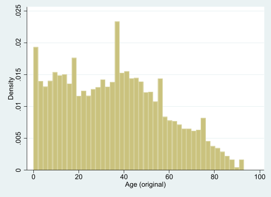
hist age, discrete(start=0, width=1)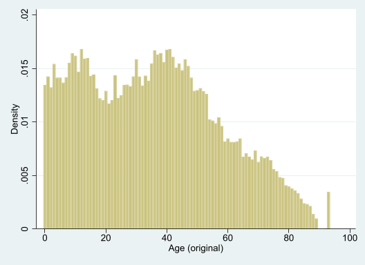
It turns out age is top-coded, and 93 really means “93 or older.” Presumably this is to preserve privacy. This could have a big impact on some forms of analysis. Of course you already know this if you read all of the codebook–always read the data documentation!
Exercise 9
“Other” is coded as 8. Hopefully you looked at several variables, but the one of interest is hispanic:
tab hispanic if race==8
  Person is |
   hispanic |      Freq.     Percent        Cum.
------------+-----------------------------------
          0 |         58        3.65        3.65
          1 |      1,529       96.35      100.00
------------+-----------------------------------
      Total |      1,587      100.00
In other words, almost all the people who marked “Other” for race are Hispanic, though not all Hispanics chose “Other”:
tab race if hispanic
            Race Recode 1 |      Freq.     Percent        Cum.
--------------------------+-----------------------------------
                    White |      1,707       48.13       48.13
                    Black |         57        1.61       49.73
          American Indian |         11        0.31       50.04
            Alaska Native |          1        0.03       50.07
Indigenous, tribe unknown |         22        0.62       50.69
                    Asian |          3        0.08       50.78
         Pacific Islander |          1        0.03       50.80
                    Other |      1,529       43.11       93.91
              Multiracial |        216        6.09      100.00
--------------------------+-----------------------------------
                    Total |      3,547      100.00
Social scientists think of “Hispanic” as an ethnicity, not a race. People who are Hispanic may be White, Black, etc. But laypeople often think of Hispanic as a race. Thus almost half of Hispanics looked at the list of available races and chose “Other” because Hispanic was not on the list. The 2010 Census tried to avoid this problem by adding a note to the instructions: “For this census, Hispanic Origins are not races.”
Excercise 11
Most children under the age of 15 probably have zero income, though some may have a small amount of income. Certainly their distribution of income is very different and generally lower than the observed distribution. If these values were observed, the mean of income would be much lower, so using the sample mean as an estimator of the population mean is biased upward by the missing data. Fortunately we’re usually interested in the income of adults.
10.3 Working With Hierarchical Data
clear
use acs
. clear

. use acs

.
Exercise 1
In this data set a level two unit is a person, a level one unit is a person-month combination (you can call it a month as long as it’s understood two people observed in the same month is two observations, not one), years_edu is a level two variable because it is always the same for a given person (it does not change over time), and employed is a level one variable because it is not always the same for a given person.
Exercise 2
by household: egen mean_age = mean(age)
list household person age mean_age in 1/5
. by household: egen mean_age = mean(age)

. list household person age mean_age in 1/5

     +------------------------------------+
     | househ~d   person   age   mean_age |
     |------------------------------------|
  1. |       37        1    20   19.33333 |
  2. |       37        2    19   19.33333 |
  3. |       37        3    19   19.33333 |
  4. |      241        1    50         50 |
  5. |      242        1    29         29 |
     +------------------------------------+

.
Exercise 3
Now the subset of interest is the adults:
gen age_if_adult = age if age>=18
by household: egen mean_adult_age = mean(age_if_adult)
list household person age mean_adult_age if household==8787, ab(30)
. gen age_if_adult = age if age>=18
(7,292 missing values generated)

. by household: egen mean_adult_age = mean(age_if_adult)
(3 missing values generated)

. list household person age mean_adult_age if household==8787, ab(30)

       +-------------------------------------------+
       | household   person   age   mean_adult_age |
       |-------------------------------------------|
  179. |      8787        1    45               45 |
  180. |      8787        2    16               45 |
  181. |      8787        3    15               45 |
       +-------------------------------------------+

.
Exercise 4
First remind yourself of the coding scheme for edu:
label list edu_labeledu_label:
0 Not in universe
1 None
2 Nursery school-4th grade
3 5th-6th grade
4 7th-8th grade
5 9th grade
6 10th grade
7 11th grade
8 12th grade, no diploma
9 High School graduate
10 Some college, <1 year
11 Some college, >=1 year
12 Associate degree
13 Bachelor's degree
14 Master's degree
15 Professional degree
16 Doctorate degreeThus someone is a college graduate if edu is greater than 11 but not missing:
gen grad = (edu>11 & edu<.)Now you’re ready to create your household-level variables:
by household: egen num_grads = total(grad)
by household: egen prop_grads = mean(grad)
by household: egen has_grad = max(grad)
list household person age edu num_grads prop_grads has_grad if household==4398, ab(30)
. by household: egen num_grads = total(grad)

. by household: egen prop_grads = mean(grad)

. by household: egen has_grad = max(grad)

. list household person age edu num_grads prop_grads has_grad if household==4398, ab(30)

       +------------------------------------------------------------------------------------+
       | household   person   age                   edu   num_grads   prop_grads   has_grad |
       |------------------------------------------------------------------------------------|
   93. |      4398        1    33   Professional degree           2           .4          1 |
   94. |      4398        2    34       Master's degree           2           .4          1 |
   95. |      4398        3     5                  None           2           .4          1 |
   96. |      4398        4     3                  None           2           .4          1 |
   97. |      4398        5     0                     .           2           .4          1 |
       +------------------------------------------------------------------------------------+

.
“All the adults in the household are college graduates” is a little trickier. One approach would be to treat this as a subsetting problem and create edu_if_adult and apply min() to it. An alternative is to focus on combining conditions. An individual makes “all the adults in the household are college graduates” false if they are an adult and not a college graduate. They do their part to make it true if they are a child or a college graduate:
by household: egen all_adults_grad = min(age<18 | edu>11)
list household person age edu all_adults_grad if household==4398, ab(30)
. by household: egen all_adults_grad = min(age<18 | edu>11)

. list household person age edu all_adults_grad if household==4398, ab(30)

       +------------------------------------------------------------------+
       | household   person   age                   edu   all_adults_grad |
       |------------------------------------------------------------------|
   93. |      4398        1    33   Professional degree                 1 |
   94. |      4398        2    34       Master's degree                 1 |
   95. |      4398        3     5                  None                 1 |
   96. |      4398        4     3                  None                 1 |
   97. |      4398        5     0                     .                 1 |
       +------------------------------------------------------------------+

.
Exercise 5
If you find this exercise difficult, you may want to read the longer introduction to loops in Stata Programming Essentials. It takes the time to explain things better.
First, load acs_wide if you haven’t already, and remind yourself how race is coded:
clear
use acs_wide

label list race_label
. clear

. use acs_wide

.
. label list race_label
race_label:
           1 White
           2 Black
           3 American Indian
           4 Alaska Native
           5 Indigenous, tribe unknown
           6 Asian
           7 Pacific Islander
           8 Other
           9 Multiracial

.
forvalues i = 1/16 {
gen black`i' = (race`i'==2) if race`i' < .
}
egen has_black_member = rowmax(black*)
egen all_black = rowmin(black*)
. forvalues i = 1/16 {
  2.     gen black`i' = (race`i'==2) if race`i' < .
  3. }
(2,779 missing values generated)
(6,191 missing values generated)
(7,876 missing values generated)
(9,355 missing values generated)
(10,115 missing values generated)
(10,388 missing values generated)
(10,484 missing values generated)
(10,531 missing values generated)
(10,544 missing values generated)
(10,554 missing values generated)
(10,557 missing values generated)
(10,564 missing values generated)
(10,564 missing values generated)
(10,564 missing values generated)
(10,564 missing values generated)

.
. egen has_black_member = rowmax(black*)

. egen all_black = rowmin(black*)

.
Just so you can be sure your variables were created properly:
tab has_black_member
tab all_black
. tab has_black_member

has_black_m |
      ember |      Freq.     Percent        Cum.
------------+-----------------------------------
          0 |      9,299       88.02       88.02
          1 |      1,266       11.98      100.00
------------+-----------------------------------
      Total |     10,565      100.00

. tab all_black

  all_black |      Freq.     Percent        Cum.
------------+-----------------------------------
          0 |      9,417       89.13       89.13
          1 |      1,148       10.87      100.00
------------+-----------------------------------
      Total |     10,565      100.00

.
10.3.1 Exercise 6
clear
use nlsy

describe
duplicates report id year
. clear

. use nlsy

.
. describe

Contains data from nlsy.dta
 Observations:       241,034
    Variables:             6                  27 Dec 2022 13:11
----------------------------------------------------------------------------------------------------
Variable      Storage   Display    Value
    name         type    format    label      Variable label
----------------------------------------------------------------------------------------------------
id              float   %9.0g                 ID# (1-12686) 79
year            int     %9.0g
year_of_birth   float   %16.0g
edu             float   %24.0g     edulabel
income          float   %9.0g
age             float   %9.0g
----------------------------------------------------------------------------------------------------
Sorted by: id  year

. duplicates report id year

Duplicates in terms of id year

--------------------------------------
   Copies | Observations       Surplus
----------+---------------------------
        1 |       241034             0
--------------------------------------

.
Since id and year uniquely identify observations, we have one row per person per year. A level 2 unit is a person, a level 1 unit is a person-year combination, and the data are in long form.
To learn more we’ll list the data for person 2 (person 1 is missing a lot) but you should look at the data browser:
list if id==2, ab(30)
        +-------------------------------------------------------+
        | id   year   year_of_birth          edu   income   age |
        |-------------------------------------------------------|
    20. |  2   1979              59    9TH GRADE     4000    20 |
    21. |  2   1980              59    9TH GRADE     5000    21 |
    22. |  2   1981              59    9TH GRADE     6000    22 |
    23. |  2   1982              59    9TH GRADE    10000    23 |
    24. |  2   1983              59    9TH GRADE    11000    24 |
        |-------------------------------------------------------|
    25. |  2   1984              59    9TH GRADE    11500    25 |
    26. |  2   1985              59   12TH GRADE    11000    26 |
    27. |  2   1986              59   12TH GRADE    14000    27 |
    28. |  2   1987              59   12TH GRADE    16000    28 |
    29. |  2   1988              59   12TH GRADE    20000    29 |
        |-------------------------------------------------------|
    30. |  2   1989              59   12TH GRADE    19000    30 |
    31. |  2   1990              59   12TH GRADE    20000    31 |
    32. |  2   1991              59   12TH GRADE    20000    32 |
    33. |  2   1992              59   12TH GRADE    22000    33 |
    34. |  2   1993              59   12TH GRADE    25000    34 |
        |-------------------------------------------------------|
    35. |  2   1994              59   12TH GRADE        0    35 |
    36. |  2   1996              59   12TH GRADE        0    37 |
    37. |  2   1998              59   12TH GRADE        0    39 |
    38. |  2   2000              59   12TH GRADE        0    41 |
        +-------------------------------------------------------+
year_of_birth is a level 2 or person-level variable (it does not change), while edu, income, and age are level 1 or year-level variables.
tab edu
                     edu |      Freq.     Percent        Cum.
-------------------------+-----------------------------------
                    NONE |         77        0.04        0.04
               1ST GRADE |         55        0.03        0.07
               2ND GRADE |          2        0.00        0.07
               3RD GRADE |        248        0.13        0.19
               4TH GRADE |        245        0.12        0.32
               5TH GRADE |        263        0.13        0.45
               6TH GRADE |        970        0.49        0.94
               7TH GRADE |      2,032        1.03        1.97
               8TH GRADE |      6,239        3.16        5.13
               9TH GRADE |     10,748        5.44       10.57
              10TH GRADE |     12,667        6.41       16.98
              11TH GRADE |     13,610        6.89       23.86
              12TH GRADE |     83,641       42.32       66.19
        1ST YEAR COLLEGE |     17,291        8.75       74.94
        2ND YEAR COLLEGE |     16,001        8.10       83.03
        3RD YEAR COLLEGE |      8,465        4.28       87.32
        4TH YEAR COLLEGE |     17,106        8.66       95.97
        5TH YEAR COLLEGE |      3,292        1.67       97.64
        6TH YEAR COLLEGE |      2,546        1.29       98.93
        7TH YEAR COLLEGE |      1,173        0.59       99.52
8TH YEAR COLLEGE OR MORE |        946        0.48      100.00
-------------------------+-----------------------------------
                   Total |    197,617      100.00
edu is labeled as a categorical variable, but the underlying values are also number of years of school (except for the last one) so you can treat it as quantitative:
tab edu, nolabel
        edu |      Freq.     Percent        Cum.
------------+-----------------------------------
          0 |         77        0.04        0.04
          1 |         55        0.03        0.07
          2 |          2        0.00        0.07
          3 |        248        0.13        0.19
          4 |        245        0.12        0.32
          5 |        263        0.13        0.45
          6 |        970        0.49        0.94
          7 |      2,032        1.03        1.97
          8 |      6,239        3.16        5.13
          9 |     10,748        5.44       10.57
         10 |     12,667        6.41       16.98
         11 |     13,610        6.89       23.86
         12 |     83,641       42.32       66.19
         13 |     17,291        8.75       74.94
         14 |     16,001        8.10       83.03
         15 |      8,465        4.28       87.32
         16 |     17,106        8.66       95.97
         17 |      3,292        1.67       97.64
         18 |      2,546        1.29       98.93
         19 |      1,173        0.59       99.52
         20 |        946        0.48      100.00
------------+-----------------------------------
      Total |    197,617      100.00
Now let’s look at person 1:
list if id==1, ab(30)
        +-------------------------------------------------------+
        | id   year   year_of_birth          edu   income   age |
        |-------------------------------------------------------|
     1. |  1   1979              58   12TH GRADE     4620    21 |
     2. |  1   1980              58            .        .    22 |
     3. |  1   1981              58   12TH GRADE     5000    23 |
     4. |  1   1982              58            .        .    24 |
     5. |  1   1983              58            .        .    25 |
        |-------------------------------------------------------|
     6. |  1   1984              58            .        .    26 |
     7. |  1   1985              58            .        .    27 |
     8. |  1   1986              58            .        .    28 |
     9. |  1   1987              58            .        .    29 |
    10. |  1   1988              58            .        .    30 |
        |-------------------------------------------------------|
    11. |  1   1989              58            .        .    31 |
    12. |  1   1990              58            .        .    32 |
    13. |  1   1991              58            .        .    33 |
    14. |  1   1992              58            .        .    34 |
    15. |  1   1993              58            .        .    35 |
        |-------------------------------------------------------|
    16. |  1   1994              58            .        .    36 |
    17. |  1   1996              58            .        .    38 |
    18. |  1   1998              58            .        .    40 |
    19. |  1   2000              58            .        .    42 |
        +-------------------------------------------------------+
Collecting longitudinal data requires tracking people down repeatedly over a period of years. When the NLSY couldn’t find a subject in a given year, they could not collect data about their education and income in that year and entered missing values. The fact that age is never missing tells us it is calculated rather than collected.
Note that many longitudinal data sets will simply not have a row for a person for a time period they could not collect data about them. Also, the NLSY is very persistent about trying to contact people even if they failed to find them in the past. Other data sets give up on people more quickly so you get a lot of attrition.
Exercise 7 {.unnumbered}
by id: gen ending_income = income[_N](97,128 missing values generated)Exercise 8
Now we’re looking for a year in which the subject’s education is 12 and their education the following year is greater than 12. But remember missing is essentially infinity and thus definitely greater than 12, so this time you have to deal with missing values explicitly:
by id: gen start_college = (edu==12 & (edu[_n+1]>12 & edu[_n+1]<.))
by id: egen times_started = total(start_college)
tab times_started
. by id: gen start_college = (edu==12 & (edu[_n+1]>12 & edu[_n+1]<.))

. by id: egen times_started = total(start_college)

. tab times_started

times_start |
         ed |      Freq.     Percent        Cum.
------------+-----------------------------------
          0 |    172,349       71.50       71.50
          1 |     68,628       28.47       99.98
          2 |         57        0.02      100.00
------------+-----------------------------------
      Total |    241,034      100.00

.
Now we have people who started college multiple times. Take a look to see why:
list id year edu start_college times_started if times_started>1, ab(30)
        +----------------------------------------------------------------+
        |   id   year                edu   start_college   times_started |
        |----------------------------------------------------------------|
 64601. | 3401   1979         11TH GRADE               0               2 |
 64602. | 3401   1980         12TH GRADE               0               2 |
 64603. | 3401   1981         12TH GRADE               0               2 |
 64604. | 3401   1982         12TH GRADE               0               2 |
 64605. | 3401   1983         12TH GRADE               0               2 |
        |----------------------------------------------------------------|
 64606. | 3401   1984         12TH GRADE               0               2 |
 64607. | 3401   1985         12TH GRADE               1               2 |
 64608. | 3401   1986   1ST YEAR COLLEGE               0               2 |
 64609. | 3401   1987   1ST YEAR COLLEGE               0               2 |
 64610. | 3401   1988   1ST YEAR COLLEGE               0               2 |
        |----------------------------------------------------------------|
 64611. | 3401   1989   1ST YEAR COLLEGE               0               2 |
 64612. | 3401   1990   1ST YEAR COLLEGE               0               2 |
 64613. | 3401   1991   1ST YEAR COLLEGE               0               2 |
 64614. | 3401   1992   1ST YEAR COLLEGE               0               2 |
 64615. | 3401   1993   1ST YEAR COLLEGE               0               2 |
        |----------------------------------------------------------------|
 64616. | 3401   1994         12TH GRADE               0               2 |
 64617. | 3401   1996         12TH GRADE               0               2 |
 64618. | 3401   1998         12TH GRADE               1               2 |
 64619. | 3401   2000   1ST YEAR COLLEGE               0               2 |
 66881. | 3521   1979          9TH GRADE               0               2 |
        |----------------------------------------------------------------|
 66882. | 3521   1980         10TH GRADE               0               2 |
 66883. | 3521   1981         11TH GRADE               0               2 |
 66884. | 3521   1982         12TH GRADE               1               2 |
 66885. | 3521   1983   1ST YEAR COLLEGE               0               2 |
 66886. | 3521   1984         12TH GRADE               1               2 |
        |----------------------------------------------------------------|
 66887. | 3521   1985   1ST YEAR COLLEGE               0               2 |
 66888. | 3521   1986   1ST YEAR COLLEGE               0               2 |
 66889. | 3521   1987   2ND YEAR COLLEGE               0               2 |
 66890. | 3521   1988   2ND YEAR COLLEGE               0               2 |
 66891. | 3521   1989   2ND YEAR COLLEGE               0               2 |
        |----------------------------------------------------------------|
 66892. | 3521   1990   2ND YEAR COLLEGE               0               2 |
 66893. | 3521   1991   2ND YEAR COLLEGE               0               2 |
 66894. | 3521   1992   2ND YEAR COLLEGE               0               2 |
 66895. | 3521   1993   2ND YEAR COLLEGE               0               2 |
 66896. | 3521   1994   2ND YEAR COLLEGE               0               2 |
        |----------------------------------------------------------------|
 66897. | 3521   1996   2ND YEAR COLLEGE               0               2 |
 66898. | 3521   1998   2ND YEAR COLLEGE               0               2 |
 66899. | 3521   2000   1ST YEAR COLLEGE               0               2 |
152077. | 8005   1979         12TH GRADE               1               2 |
152078. | 8005   1980   1ST YEAR COLLEGE               0               2 |
        |----------------------------------------------------------------|
152079. | 8005   1981         12TH GRADE               0               2 |
152080. | 8005   1982         12TH GRADE               0               2 |
152081. | 8005   1983         12TH GRADE               1               2 |
152082. | 8005   1984   1ST YEAR COLLEGE               0               2 |
152083. | 8005   1985   1ST YEAR COLLEGE               0               2 |
        |----------------------------------------------------------------|
152084. | 8005   1986   1ST YEAR COLLEGE               0               2 |
152085. | 8005   1987   1ST YEAR COLLEGE               0               2 |
152086. | 8005   1988   1ST YEAR COLLEGE               0               2 |
152087. | 8005   1989   1ST YEAR COLLEGE               0               2 |
152088. | 8005   1990   1ST YEAR COLLEGE               0               2 |
        |----------------------------------------------------------------|
152089. | 8005   1991   1ST YEAR COLLEGE               0               2 |
152090. | 8005   1992   1ST YEAR COLLEGE               0               2 |
152091. | 8005   1993   1ST YEAR COLLEGE               0               2 |
152092. | 8005   1994   1ST YEAR COLLEGE               0               2 |
152093. | 8005   1996   1ST YEAR COLLEGE               0               2 |
        |----------------------------------------------------------------|
152094. | 8005   1998   1ST YEAR COLLEGE               0               2 |
152095. | 8005   2000   1ST YEAR COLLEGE               0               2 |
        +----------------------------------------------------------------+
In both cases the subject reported “1ST YEAR COLLEGE” for their education for a while, then when back to reporting “12TH GRADE” for a while before reporting college again. That’s a problem with the data, not your code, but you may need to change your code to deal with it.
Exercise 9
Two options:
gen age25 = (age==25)
sort id age25
by id: gen income25a = income[_N] if age25[_N]
sort id year

gen income_if_25 = income if age==25
by id: egen income25b = mean(income_if_25)

assert income25a==income25b
. gen age25 = (age==25)

. sort id age25

. by id: gen income25a = income[_N] if age25[_N]
(22,686 missing values generated)

. sort id year

.
. gen income_if_25 = income if age==25
(229,542 missing values generated)

. by id: egen income25b = mean(income_if_25)
(22,686 missing values generated)

.
. assert income25a==income25b

.
The assert command tells us they give exactly the same results.
10.4 Restructuring Data
Exercise 1
clear
use nlsy

duplicates report id year
list in 1/6, ab(30)
. clear

. use nlsy

.
. duplicates report id year

Duplicates in terms of id year

--------------------------------------
   Copies | Observations       Surplus
----------+---------------------------
        1 |       241034             0
--------------------------------------

. list in 1/6, ab(30)

     +-------------------------------------------------------+
     | id   year   year_of_birth          edu   income   age |
     |-------------------------------------------------------|
  1. |  1   1979              58   12TH GRADE     4620    21 |
  2. |  1   1980              58            .        .    22 |
  3. |  1   1981              58   12TH GRADE     5000    23 |
  4. |  1   1982              58            .        .    24 |
  5. |  1   1983              58            .        .    25 |
     |-------------------------------------------------------|
  6. |  1   1984              58            .        .    26 |
     +-------------------------------------------------------+

.
The unique identifiers are id and year, telling us we have one observation per person (id) per year. A person-year combination (or just year) is a level one unit, and a person is a level two unit. Looking at a few observations we see that year_of_birth is a level two variable (it does not change over time) and edu, income, and age are level one variables.
duplicates report id
reshape wide edu income age, i(id) j(year)
reshape long edu income age, i(id) j(year)
duplicates report id
. duplicates report id

Duplicates in terms of id

--------------------------------------
   Copies | Observations       Surplus
----------+---------------------------
       19 |       241034        228348
--------------------------------------

. reshape wide edu income age, i(id) j(year)
(j = 1979 1980 1981 1982 1983 1984 1985 1986 1987 1988 1989 1990 1991 1992 1993 1994 1996 1998 2000)

Data                               Long   ->   Wide
-----------------------------------------------------------------------------
Number of observations          241,034   ->   12,686
Number of variables                   6   ->   59
j variable (19 values)             year   ->   (dropped)
xij variables:
                                    edu   ->   edu1979 edu1980 ... edu2000
                                 income   ->   income1979 income1980 ... income2000
                                    age   ->   age1979 age1980 ... age2000
-----------------------------------------------------------------------------

. reshape long edu income age, i(id) j(year)
(j = 1979 1980 1981 1982 1983 1984 1985 1986 1987 1988 1989 1990 1991 1992 1993 1994 1996 1998 2000)

Data                               Wide   ->   Long
-----------------------------------------------------------------------------
Number of observations           12,686   ->   241,034
Number of variables                  59   ->   6
j variable (19 values)                    ->   year
xij variables:
            edu1979 edu1980 ... edu2000   ->   edu
   income1979 income1980 ... income2000   ->   income
            age1979 age1980 ... age2000   ->   age
-----------------------------------------------------------------------------

. duplicates report id

Duplicates in terms of id

--------------------------------------
   Copies | Observations       Surplus
----------+---------------------------
       19 |       241034        228348
--------------------------------------

.
This data set starts with exactly 19 observations for each person. Even if the NLSY researchers could not find a person in a given year, they created an observation for them with missing data. Thus, unlike the ACS, no new observations are created when the data set is reshaped from wide to long.
Exercise 2
clear
use nlsy

collapse ///
    (first) year_of_birth ///
    (mean) income ///
    (max) edu, ///
    by(id)

l in 1/5, ab(30)
. clear

. use nlsy

.
. collapse ///
>     (first) year_of_birth ///
>     (mean) income ///
>     (max) edu, ///
>     by(id)

.
. l in 1/5, ab(30)

     +-------------------------------------+
     | id   year_of_birth     income   edu |
     |-------------------------------------|
  1. |  1              58       4810    12 |
  2. |  2              59   11289.47    12 |
  3. |  3              61   4735.294    12 |
  4. |  4              62      12874    14 |
  5. |  5              59      20631    18 |
     +-------------------------------------+

.
Aggregating income across multiple decades without correcting for inflation is a very bad idea, but you’ll learn how to correct for inflation as an example in the next chapter.
10.5 Combining Data Sets
Exercise 1
acs_race.dta and acs_education.dta contain different variables for the same people (open them and look at the data browser), so they need to be merged.
clear
use acs_race
merge 1:1  household person using acs_education
. clear

. use acs_race

. merge 1:1  household person using acs_education

    Result                      Number of obs
    -----------------------------------------
    Not matched                             0
    Matched                            27,410  (_merge==3)
    -----------------------------------------

.
acs_adults.dta and acs_children.dta contain the same variables for different people, so they need to be appended.
clear
use acs_adults
append using acs_children
. clear

. use acs_adults

. append using acs_children
(label edu_label already defined)
(label race_label already defined)
(label marital_status_label already defined)

.
Exercise 2
First take a look at the data sets in the data browser and note the data structure. For the book we’ll skip to confirming the identifiers.
clear
use nlsy7980
duplicates report id year
. clear

. use nlsy7980

. duplicates report id year

Duplicates in terms of id year

--------------------------------------
   Copies | Observations       Surplus
----------+---------------------------
        1 |        25372             0
--------------------------------------

.
nlsy7980 has one observation per person (id) per year, so it’s in long form.
clear
use nlsy8182
duplicates report id
describe
. clear

. use nlsy8182

. duplicates report id

Duplicates in terms of id

--------------------------------------
   Copies | Observations       Surplus
----------+---------------------------
        1 |        12686             0
--------------------------------------

. describe

Contains data from nlsy8182.dta
 Observations:        12,686
    Variables:             8                  27 Dec 2022 13:13
----------------------------------------------------------------------------------------------------
Variable      Storage   Display    Value
    name         type    format    label      Variable label
----------------------------------------------------------------------------------------------------
id              float   %9.0g                 ID# (1-12686) 79
edu1981         float   %24.0g     edulabel   1981 edu
income1981      float   %9.0g                 1981 income
age1981         float   %9.0g                 1981 age
edu1982         float   %24.0g     edulabel   1982 edu
income1982      float   %9.0g                 1982 income
age1982         float   %9.0g                 1982 age
year_of_birth   float   %16.0g
----------------------------------------------------------------------------------------------------
Sorted by: id

.
nlsy8182 has one observation per person and one set of variables per year, so it’s in wide form. Before we can combine these data sets we must put them in the same form.
If you want the result to be in long form, them you need to reshape nlsy8182 to long form and then use append:
reshape long edu income age, i(id) j(year)
append using nlsy7980
describe
. reshape long edu income age, i(id) j(year)
(j = 1981 1982)

Data                               Wide   ->   Long
-----------------------------------------------------------------------------
Number of observations           12,686   ->   25,372
Number of variables                   8   ->   6
j variable (2 values)                     ->   year
xij variables:
                        edu1981 edu1982   ->   edu
                  income1981 income1982   ->   income
                        age1981 age1982   ->   age
-----------------------------------------------------------------------------

. append using nlsy7980
(label edulabel already defined)

. describe

Contains data
 Observations:        50,744
    Variables:             6
----------------------------------------------------------------------------------------------------
Variable      Storage   Display    Value
    name         type    format    label      Variable label
----------------------------------------------------------------------------------------------------
id              float   %9.0g                 ID# (1-12686) 79
year            int     %10.0g
edu             float   %24.0g     edulabel
income          float   %9.0g
age             float   %9.0g
year_of_birth   float   %16.0g
----------------------------------------------------------------------------------------------------
Sorted by:
     Note: Dataset has changed since last saved.

.
If you want the result to be in wide form, you must reshape nlsy7980 to wide form and then use merge:
clear
use nlsy7980
reshape wide edu income age, i(id) j(year)
merge 1:1 id using nlsy8182
describe
. clear

. use nlsy7980

. reshape wide edu income age, i(id) j(year)
(j = 1979 1980)

Data                               Long   ->   Wide
-----------------------------------------------------------------------------
Number of observations           25,372   ->   12,686
Number of variables                   6   ->   8
j variable (2 values)              year   ->   (dropped)
xij variables:
                                    edu   ->   edu1979 edu1980
                                 income   ->   income1979 income1980
                                    age   ->   age1979 age1980
-----------------------------------------------------------------------------

. merge 1:1 id using nlsy8182
(label edulabel already defined)

    Result                      Number of obs
    -----------------------------------------
    Not matched                             0
    Matched                            12,686  (_merge==3)
    -----------------------------------------

. describe

Contains data
 Observations:        12,686
    Variables:            15
----------------------------------------------------------------------------------------------------
Variable      Storage   Display    Value
    name         type    format    label      Variable label
----------------------------------------------------------------------------------------------------
id              float   %9.0g                 ID# (1-12686) 79
edu1979         float   %24.0g     edulabel   1979 edu
income1979      float   %9.0g                 1979 income
age1979         float   %9.0g                 1979 age
edu1980         float   %24.0g     edulabel   1980 edu
income1980      float   %9.0g                 1980 income
age1980         float   %9.0g                 1980 age
year_of_birth   float   %16.0g
edu1981         float   %24.0g     edulabel   1981 edu
income1981      float   %9.0g                 1981 income
age1981         float   %9.0g                 1981 age
edu1982         float   %24.0g     edulabel   1982 edu
income1982      float   %9.0g                 1982 income
age1982         float   %9.0g                 1982 age
_merge          byte    %23.0g     _merge     Matching result from merge
----------------------------------------------------------------------------------------------------
Sorted by: id
     Note: Dataset has changed since last saved.

.
Exercise 3
clear
use nlsy_person
merge 1:m id using nlsy_person_year
. clear

. use nlsy_person

. merge 1:m id using nlsy_person_year

    Result                      Number of obs
    -----------------------------------------
    Not matched                             0
    Matched                           241,034  (_merge==3)
    -----------------------------------------

.
Exercise 4
First take a look at the problem:
clear
use nlsy_error
duplicates report id year
bysort id year: gen copies = _N
list if copies>1, ab(30)
. clear

. use nlsy_error

. duplicates report id year

Duplicates in terms of id year

--------------------------------------
   Copies | Observations       Surplus
----------+---------------------------
        1 |       240974             0
        2 |           80            40
--------------------------------------

. bysort id year: gen copies = _N

. list if copies>1, ab(30)

        +------------------------------------------------------------------------+
        |   id   year   year_of_birth                edu   income   age   copies |
        |------------------------------------------------------------------------|
  9507. |  501   1985              63   3RD YEAR COLLEGE     3000    22        2 |
  9508. |  501   1985              63   3RD YEAR COLLEGE     3000    22        2 |
 26450. | 1393   1979              58         12TH GRADE     7000    21        2 |
 26451. | 1393   1979              58         12TH GRADE     7000    21        2 |
 26452. | 1393   1980              58         12TH GRADE     7000    22        2 |
        |------------------------------------------------------------------------|
 26453. | 1393   1980              58         12TH GRADE     7000    22        2 |
 26454. | 1393   1981              58         12TH GRADE     7000    23        2 |
 26455. | 1393   1981              58         12TH GRADE     7000    23        2 |
 26456. | 1393   1982              58         12TH GRADE     6000    24        2 |
 26457. | 1393   1982              58         12TH GRADE     6000    24        2 |
        |------------------------------------------------------------------------|
 26458. | 1393   1983              58         12TH GRADE    31519    25        2 |
 26459. | 1393   1983              58         12TH GRADE    31519    25        2 |
 26460. | 1393   1984              58         12TH GRADE    22000    26        2 |
 26461. | 1393   1984              58         12TH GRADE    22000    26        2 |
 26462. | 1393   1985              58         12TH GRADE    39389    27        2 |
        |------------------------------------------------------------------------|
 26463. | 1393   1985              58         12TH GRADE    39389    27        2 |
 26464. | 1393   1986              58         12TH GRADE    43119    28        2 |
 26465. | 1393   1986              58         12TH GRADE    43119    28        2 |
 26466. | 1393   1987              58         12TH GRADE    10000    29        2 |
 26467. | 1393   1987              58         12TH GRADE    10000    29        2 |
        |------------------------------------------------------------------------|
 26468. | 1393   1988              58         12TH GRADE    20000    30        2 |
 26469. | 1393   1988              58         12TH GRADE    20000    30        2 |
 26470. | 1393   1989              58         12TH GRADE    25000    31        2 |
 26471. | 1393   1989              58         12TH GRADE    25000    31        2 |
 26472. | 1393   1990              58         12TH GRADE    31000    32        2 |
        |------------------------------------------------------------------------|
 26473. | 1393   1990              58         12TH GRADE    31000    32        2 |
 26474. | 1393   1991              58         12TH GRADE    40000    33        2 |
 26475. | 1393   1991              58         12TH GRADE    40000    33        2 |
 26476. | 1393   1992              58         12TH GRADE    32000    34        2 |
 26477. | 1393   1992              58         12TH GRADE    32000    34        2 |
        |------------------------------------------------------------------------|
 26478. | 1393   1993              58         12TH GRADE    49000    35        2 |
 26479. | 1393   1993              58         12TH GRADE    49000    35        2 |
 26480. | 1393   1994              58         12TH GRADE    58000    36        2 |
 26481. | 1393   1994              58         12TH GRADE    58000    36        2 |
 26482. | 1393   1996              58   1ST YEAR COLLEGE    43000    38        2 |
        |------------------------------------------------------------------------|
 26483. | 1393   1996              58   1ST YEAR COLLEGE    43000    38        2 |
 26484. | 1393   1998              58   1ST YEAR COLLEGE    58000    40        2 |
 26485. | 1393   1998              58   1ST YEAR COLLEGE    58000    40        2 |
 26486. | 1393   2000              58   3RD YEAR COLLEGE    40000    42        2 |
 26487. | 1393   2000              58   3RD YEAR COLLEGE    40000    42        2 |
        |------------------------------------------------------------------------|
 38971. | 2051   1979              64          7TH GRADE        .    15        2 |
 38972. | 2051   1979              64          8TH GRADE        .    15        2 |
 38973. | 2051   1980              64                  .        .    16        2 |
 38974. | 2051   1980              64          8TH GRADE        .    16        2 |
 38975. | 2051   1981              64                  .        .    17        2 |
        |------------------------------------------------------------------------|
 38976. | 2051   1981              64          9TH GRADE        .    17        2 |
 38977. | 2051   1982              64         10TH GRADE        .    18        2 |
 38978. | 2051   1982              64                  .        .    18        2 |
 38979. | 2051   1983              64         11TH GRADE     2180    19        2 |
 38980. | 2051   1983              64         12TH GRADE     1500    19        2 |
        |------------------------------------------------------------------------|
 38981. | 2051   1984              64   1ST YEAR COLLEGE     2000    20        2 |
 38982. | 2051   1984              64         11TH GRADE     4500    20        2 |
 38983. | 2051   1985              64   2ND YEAR COLLEGE     2000    21        2 |
 38984. | 2051   1985              64         11TH GRADE     5546    21        2 |
 38985. | 2051   1986              64         11TH GRADE    10000    22        2 |
        |------------------------------------------------------------------------|
 38986. | 2051   1986              64   2ND YEAR COLLEGE     3000    22        2 |
 38987. | 2051   1987              64   3RD YEAR COLLEGE     6400    23        2 |
 38988. | 2051   1987              64         11TH GRADE    11000    23        2 |
 38989. | 2051   1988              64   4TH YEAR COLLEGE    12000    24        2 |
 38990. | 2051   1988              64         11TH GRADE     7000    24        2 |
        |------------------------------------------------------------------------|
 38991. | 2051   1989              64         11TH GRADE     2500    25        2 |
 38992. | 2051   1989              64   4TH YEAR COLLEGE    22000    25        2 |
 38993. | 2051   1990              64         11TH GRADE     9000    26        2 |
 38994. | 2051   1990              64                  .        .    26        2 |
 38995. | 2051   1991              64   4TH YEAR COLLEGE    28000    27        2 |
        |------------------------------------------------------------------------|
 38996. | 2051   1991              64         11TH GRADE     8556    27        2 |
 38997. | 2051   1992              64   4TH YEAR COLLEGE    28000    28        2 |
 38998. | 2051   1992              64         11TH GRADE    10000    28        2 |
 38999. | 2051   1993              64   4TH YEAR COLLEGE    30000    29        2 |
 39000. | 2051   1993              64         11TH GRADE    14000    29        2 |
        |------------------------------------------------------------------------|
 39001. | 2051   1994              64   4TH YEAR COLLEGE    39000    30        2 |
 39002. | 2051   1994              64         11TH GRADE    13000    30        2 |
 39003. | 2051   1996              64   4TH YEAR COLLEGE    55000    32        2 |
 39004. | 2051   1996              64         11TH GRADE    15000    32        2 |
 39005. | 2051   1998              64         11TH GRADE    17751    34        2 |
        |------------------------------------------------------------------------|
 39006. | 2051   1998              64   4TH YEAR COLLEGE    60000    34        2 |
 39007. | 2051   2000              64                  .        .    36        2 |
 39008. | 2051   2000              64         11TH GRADE    30000    36        2 |
123731. | 6512   1980              57         12TH GRADE        0    23        2 |
123732. | 6512   1980              57         12TH GRADE     2900    24        2 |
        +------------------------------------------------------------------------+

.
Some of these are completely duplicate observations which can be remedied with duplicates drop:
duplicates drop
Duplicates in terms of all variables

(20 observations deleted)
Now examine the remaining problems:
by id year: replace copies = _N
list if copies>1, ab(30)
. by id year: replace copies = _N
(20 real changes made)

. list if copies>1, ab(30)

        +------------------------------------------------------------------------+
        |   id   year   year_of_birth                edu   income   age   copies |
        |------------------------------------------------------------------------|
 38951. | 2051   1979              64          7TH GRADE        .    15        2 |
 38952. | 2051   1979              64          8TH GRADE        .    15        2 |
 38953. | 2051   1980              64                  .        .    16        2 |
 38954. | 2051   1980              64          8TH GRADE        .    16        2 |
 38955. | 2051   1981              64                  .        .    17        2 |
        |------------------------------------------------------------------------|
 38956. | 2051   1981              64          9TH GRADE        .    17        2 |
 38957. | 2051   1982              64         10TH GRADE        .    18        2 |
 38958. | 2051   1982              64                  .        .    18        2 |
 38959. | 2051   1983              64         11TH GRADE     2180    19        2 |
 38960. | 2051   1983              64         12TH GRADE     1500    19        2 |
        |------------------------------------------------------------------------|
 38961. | 2051   1984              64   1ST YEAR COLLEGE     2000    20        2 |
 38962. | 2051   1984              64         11TH GRADE     4500    20        2 |
 38963. | 2051   1985              64   2ND YEAR COLLEGE     2000    21        2 |
 38964. | 2051   1985              64         11TH GRADE     5546    21        2 |
 38965. | 2051   1986              64         11TH GRADE    10000    22        2 |
        |------------------------------------------------------------------------|
 38966. | 2051   1986              64   2ND YEAR COLLEGE     3000    22        2 |
 38967. | 2051   1987              64   3RD YEAR COLLEGE     6400    23        2 |
 38968. | 2051   1987              64         11TH GRADE    11000    23        2 |
 38969. | 2051   1988              64   4TH YEAR COLLEGE    12000    24        2 |
 38970. | 2051   1988              64         11TH GRADE     7000    24        2 |
        |------------------------------------------------------------------------|
 38971. | 2051   1989              64         11TH GRADE     2500    25        2 |
 38972. | 2051   1989              64   4TH YEAR COLLEGE    22000    25        2 |
 38973. | 2051   1990              64         11TH GRADE     9000    26        2 |
 38974. | 2051   1990              64                  .        .    26        2 |
 38975. | 2051   1991              64   4TH YEAR COLLEGE    28000    27        2 |
        |------------------------------------------------------------------------|
 38976. | 2051   1991              64         11TH GRADE     8556    27        2 |
 38977. | 2051   1992              64   4TH YEAR COLLEGE    28000    28        2 |
 38978. | 2051   1992              64         11TH GRADE    10000    28        2 |
 38979. | 2051   1993              64   4TH YEAR COLLEGE    30000    29        2 |
 38980. | 2051   1993              64         11TH GRADE    14000    29        2 |
        |------------------------------------------------------------------------|
 38981. | 2051   1994              64   4TH YEAR COLLEGE    39000    30        2 |
 38982. | 2051   1994              64         11TH GRADE    13000    30        2 |
 38983. | 2051   1996              64   4TH YEAR COLLEGE    55000    32        2 |
 38984. | 2051   1996              64         11TH GRADE    15000    32        2 |
 38985. | 2051   1998              64         11TH GRADE    17751    34        2 |
        |------------------------------------------------------------------------|
 38986. | 2051   1998              64   4TH YEAR COLLEGE    60000    34        2 |
 38987. | 2051   2000              64                  .        .    36        2 |
 38988. | 2051   2000              64         11TH GRADE    30000    36        2 |
123711. | 6512   1980              57         12TH GRADE        0    23        2 |
123712. | 6512   1980              57         12TH GRADE     2900    24        2 |
        +------------------------------------------------------------------------+

.
The remaining observations are not duplicates and suggest different people were assigned the same id by accident. For real work you might investigate further, including contacting the data provider, but for now you can eliminate all the problem observations with:
drop if copies>1(40 observations deleted)Now you could run a one-to-one merge using id and year:
duplicates report id year
Duplicates in terms of id year

--------------------------------------
   Copies | Observations       Surplus
----------+---------------------------
        1 |       240994             0
--------------------------------------
10.6 Learning More
clear
sysuse auto
gen company = word(make, 1)
gen model = subinstr(make, company + " ", "", 1)
list make company model
. clear

. sysuse auto
(1978 automobile data)

. gen company = word(make, 1)

. gen model = subinstr(make, company + " ", "", 1)

. list make company model

     +-------------------------------------------+
     | make                company         model |
     |-------------------------------------------|
  1. | AMC Concord             AMC       Concord |
  2. | AMC Pacer               AMC         Pacer |
  3. | AMC Spirit              AMC        Spirit |
  4. | Buick Century         Buick       Century |
  5. | Buick Electra         Buick       Electra |
     |-------------------------------------------|
  6. | Buick LeSabre         Buick       LeSabre |
  7. | Buick Opel            Buick          Opel |
  8. | Buick Regal           Buick         Regal |
  9. | Buick Riviera         Buick       Riviera |
 10. | Buick Skylark         Buick       Skylark |
     |-------------------------------------------|
 11. | Cad. Deville           Cad.       Deville |
 12. | Cad. Eldorado          Cad.      Eldorado |
 13. | Cad. Seville           Cad.       Seville |
 14. | Chev. Chevette        Chev.      Chevette |
 15. | Chev. Impala          Chev.        Impala |
     |-------------------------------------------|
 16. | Chev. Malibu          Chev.        Malibu |
 17. | Chev. Monte Carlo     Chev.   Monte Carlo |
 18. | Chev. Monza           Chev.         Monza |
 19. | Chev. Nova            Chev.          Nova |
 20. | Dodge Colt            Dodge          Colt |
     |-------------------------------------------|
 21. | Dodge Diplomat        Dodge      Diplomat |
 22. | Dodge Magnum          Dodge        Magnum |
 23. | Dodge St. Regis       Dodge     St. Regis |
 24. | Ford Fiesta            Ford        Fiesta |
 25. | Ford Mustang           Ford       Mustang |
     |-------------------------------------------|
 26. | Linc. Continental     Linc.   Continental |
 27. | Linc. Mark V          Linc.        Mark V |
 28. | Linc. Versailles      Linc.    Versailles |
 29. | Merc. Bobcat          Merc.        Bobcat |
 30. | Merc. Cougar          Merc.        Cougar |
     |-------------------------------------------|
 31. | Merc. Marquis         Merc.       Marquis |
 32. | Merc. Monarch         Merc.       Monarch |
 33. | Merc. XR-7            Merc.          XR-7 |
 34. | Merc. Zephyr          Merc.        Zephyr |
 35. | Olds 98                Olds            98 |
     |-------------------------------------------|
 36. | Olds Cutl Supr         Olds     Cutl Supr |
 37. | Olds Cutlass           Olds       Cutlass |
 38. | Olds Delta 88          Olds      Delta 88 |
 39. | Olds Omega             Olds         Omega |
 40. | Olds Starfire          Olds      Starfire |
     |-------------------------------------------|
 41. | Olds Toronado          Olds      Toronado |
 42. | Plym. Arrow           Plym.         Arrow |
 43. | Plym. Champ           Plym.         Champ |
 44. | Plym. Horizon         Plym.       Horizon |
 45. | Plym. Sapporo         Plym.       Sapporo |
     |-------------------------------------------|
 46. | Plym. Volare          Plym.        Volare |
 47. | Pont. Catalina        Pont.      Catalina |
 48. | Pont. Firebird        Pont.      Firebird |
 49. | Pont. Grand Prix      Pont.    Grand Prix |
 50. | Pont. Le Mans         Pont.       Le Mans |
     |-------------------------------------------|
 51. | Pont. Phoenix         Pont.       Phoenix |
 52. | Pont. Sunbird         Pont.       Sunbird |
 53. | Audi 5000              Audi          5000 |
 54. | Audi Fox               Audi           Fox |
 55. | BMW 320i                BMW          320i |
     |-------------------------------------------|
 56. | Datsun 200           Datsun           200 |
 57. | Datsun 210           Datsun           210 |
 58. | Datsun 510           Datsun           510 |
 59. | Datsun 810           Datsun           810 |
 60. | Fiat Strada            Fiat        Strada |
     |-------------------------------------------|
 61. | Honda Accord          Honda        Accord |
 62. | Honda Civic           Honda         Civic |
 63. | Mazda GLC             Mazda           GLC |
 64. | Peugeot 604         Peugeot           604 |
 65. | Renault Le Car      Renault        Le Car |
     |-------------------------------------------|
 66. | Subaru               Subaru        Subaru |
 67. | Toyota Celica        Toyota        Celica |
 68. | Toyota Corolla       Toyota       Corolla |
 69. | Toyota Corona        Toyota        Corona |
 70. | VW Dasher                VW        Dasher |
     |-------------------------------------------|
 71. | VW Diesel                VW        Diesel |
 72. | VW Rabbit                VW        Rabbit |
 73. | VW Scirocco              VW      Scirocco |
 74. | Volvo 260             Volvo           260 |
     +-------------------------------------------+

.