capture log close
log using combine.do
clear all6 Combining Data Sets
Combining data sets is a very common task, and one that’s easy to do if you understand the structure of the data sets you are trying to combine. However, if you’ve misunderstood the structure of the data sets you can end up with a data set that makes no sense at all. Also, combining data sets will often force you to deal with problems in the data set structure.
Stata always works with one data set. (Stata recently added the ability to load multiple data sets as separate frames, but we won’t explore this new feature.) So when we talk about combining data sets we mean taking a data set that’s in memory, what Stata calls the master data set, and combining it with a data set on disk, what Stata calls the using data set for reasons that will become obvious when you see the command syntax. When you’re done, you’ll have a single data set in memory again.
Always think through what the resulting data set should look like before combining two data sets. If the resulting data set won’t have a consistent, logical structure you probably need to rethink what you’re doing.
How you combine the two data sets depends on what the using data set adds to the master data set. We’ll discuss the most common scenarios, which are:
- Adding observations
- Adding variables
- Adding level one units to existing level two units
- Adding variables for different levels
6.1 Setting Up
Start a do file called combine.do. Don’t worry about loading any data yet–in this chapter almost every example will involve different data sets.
6.2 Adding Observations
If the using data set adds more observations to the master data set, then this is a job for append. Using append makes sense if the master data set and the using data set contain the same kinds of things, but not the same things. The append command simply adds the using data set to the end of the master data set.
Suppose that instead of a single file containing ACS sample you were given acs_part1.dta and acs_part2.dta, with each file containing about half of the observations. Load acs_part1, then use append to add acs_part2, combining them into a single data set:
use acs_part1
append using acs_part2
If a variable only exists in one of the two data sets, observations from the other data set will have missing values for that variable. Make sure variables have the same name in both files before appending them, or append will treat them as different variables. Of course that assumes they actually measure the same thing in the same way. The warning you got about labels already being defined tells you those variables have value labels defined in both files, and you should make sure that they agree about what the values mean.
6.3 Adding Variables
If the using data set adds more variables to the master data set and observations represent the same things in both data sets, then this is a job for a one-to-one merge. The merge command combines data sets by combining observations that have the same value of an identifier variable or variables, so the result has all the variables from both files.
Suppose you were given the data files acs_demographics.dta and acs_ses.dta, containing demographic information and socio-economic status (SES) information respectively about the ACS respondents. You can use merge to combine them into a single data set:
clear
use acs_demographics
merge 1:1 household person using acs_ses
. clear

. use acs_demographics

. merge 1:1 household person using acs_ses

    Result                      Number of obs
    -----------------------------------------
    Not matched                             0
    Matched                            27,410  (_merge==3)
    -----------------------------------------

.
1:1 means you are doing a one-to-one merge: one respondent’s demographic information will be matched with one respondent’s SES information. Next come the identifier variables, two in this case, that tell merge which observations should be matched. Because we’ve specified that this is a 1:1 merge, the identifier variable(s) must uniquely identify observations in both data sets. We’ll talk about handling duplicate identifiers shortly. The identifier variables must exist in both data sets, and have the same names, but in most cases all of the other variables should have different names.
If an observation in one data set does not match anything in the other data set, it will get missing values for all the variables in that data set. How successful you are at matching observations can sometimes affect your entire research agenda, so Stata both gives you a report and creates a new variable, _merge, that tells you whether a given observation matched or not. In this case, all the observations matched and thus got a 3 for _merge. A 1 means the observation came from the master data but did not match anything in the using data set; a 2 means the observation came from the using data set but did not match anything in the master data set. Note that you cannot carry out another merge until you drop or rename the _merge variable so Stata can create a new one.
Exercise 1
Examine the following pairs of data sets: acs_race.dta and acs_education.dta; acs_adults.dta and acs_children.dta. Determine the appropriate method for combining each pair into a single data set and then do so.
6.4 Adding Level One Units to Existing Level Two Units
Next consider the data sets nlsy1979.dta and nlsy1980.dta. They each contain one year’s worth of data from our NLSY extract. Is combining them a job for append or for merge?
The answer depends on whether you want the resulting data set to be in long form or in wide form. In the NLSY, a level two unit is a person and a level one unit is a person-year combination, so adding nlsy1980 to nlsy1979 is adding new level one units (years) to the existing level two units (people). In long form each level one unit gets its own observation, so adding nlsy1980 in long form adds observations. This is a job for append. In wide form, each level two unit gets its own observation, but each level one unit gets its own set of variables. Thus adding nlsy1980 in wide form adds variables; a job for merge.
The only complication is the level one identifier, year. Right now it is found only in the filenames of the two data sets, as is common. In long form, the level one identifier needs to be a variable. In wide form, it needs to be a suffix at the end of the names of all the level one variables. Either way that needs to be done before combining the data sets, or you’ll have no way of knowing whether a value is from 1979 or 1980.
First combine the two files using append so the result is in long form. Begin by loading nlsy1980, creating a year variable set to 1980, and saving the results:
clear
use nlsy1980
gen year=1980
save nlsy1980_append, replace
. clear

. use nlsy1980

. gen year=1980

. save nlsy1980_append, replace
file nlsy1980_append.dta saved

.
Next, load nlsy1979 and create a year variable set to 1979:
use nlsy1979
gen year=1979
. use nlsy1979

. gen year=1979

.
Now combine them with append:
append using nlsy1980_append(label edulabel already defined)This will give you a dataset with first all the 1979 observations and then all the 1980 observations. It’s often useful to have all the observations for a given person together and in chronological order, which you could get by running sort id year.
Now combine the two files using merge so the result is in wide form. Begin by loading nlsy1980, but this time instead of creating a variable to store 1980 we need to add 1980 to the names of all the level one variables: edu, income, and age. You could do that with three rename commands (e.g. rename edu edu1980) but you can also rename them as a group:
clear
use nlsy1980
rename edu-age =1980
save nlsy1980_merge, replace
. clear

. use nlsy1980

. rename edu-age =1980

. save nlsy1980_merge, replace
file nlsy1980_merge.dta saved

.
This rename command first uses variable list syntax to specify the variables to be acted on, edu-age, and then specifies that 1980 should be added to the end of the existing variable names with =1980.
Repeat the process for nlsy1979:
use nlsy1979
rename edu-age =1979
. use nlsy1979

. rename edu-age =1979

.
Now you’re ready to combine them with merge. This will again be a one-to-one merge, since one person’s data from 1979 is being combined with one person’s data from 1980.
merge 1:1 id using nlsy1980_merge(label edulabel already defined)
Result Number of obs
-----------------------------------------
Not matched 0
Matched 12,686 (_merge==3)
-----------------------------------------Exercise 2
The files nlsy7980.dta and nlsy8182.dta each contain two level one units (person-year combinations). Combine them into either long form or wide form, using reshape to make them consistent before combining.
6.5 Adding Variables for Different Levels
If you need to combine hierarchical data where the master data set contains data on the level one units and the using data set contains data on the level two units, this is a job for a many-to-one merge. A many-to-one merge combines observations just like a one-to-one merge, but many level one units are combined with one level two unit. A one-to-many merge is essentially the same thing, just the master data set contains the level two unit (the “one”) and the using data set contains the level one units (the “many”).
The data set acs_households.dta contains information about the households in our 2000 ACS extract (in particular, their household income). There is one observation per household. Adding it to acs.dta is a job for a many-to-one merge:
clear
use acs
merge m:1 household using acs_households
. clear

. use acs

. merge m:1 household using acs_households

    Result                      Number of obs
    -----------------------------------------
    Not matched                             0
    Matched                            27,410  (_merge==3)
    -----------------------------------------

.
Note that the key variable here is just household, not household and person like in prior merges.
You can also combine these data sets by adding acs to acs_households. This will be a one-to-many merge but the result will be the same:
clear
use acs_households
merge 1:m household using acs
. clear

. use acs_households

. merge 1:m household using acs

    Result                      Number of obs
    -----------------------------------------
    Not matched                             0
    Matched                            27,410  (_merge==3)
    -----------------------------------------

.
Exercise 3
nlsy_person contains information about the people in our NLSY extract that does not change over time, while nlsy_person_year contains only variables that change from year to year. Combine them.
6.6 Adjusting for Inflation
Next we’ll do an example that illustrates some of the issues that frequently arise when combining data sets from different sources.
One weakness of the NLSY data extract we’ve been using is that incomes from different time periods are not really comparable, due to inflation. To adjust them for inflation, we need information about the level of inflation in each year. The fredcpi data set contains the average Consumer Price Index for All Urban Consumers for every year from 1970 to 2019. It was obtained from the Federal Reserve Economic Data (FRED). If you have a FRED API key, and if you are interested in the US economy you probably want one, you can obtain it directly from FRED with:
import fred CPIAUCSL, daterange(1970 2019) aggregate(annual,avg)If you click File, Import, Federal Reserve Economic Data (FRED) you can search for and download a variety of economic data.
Taking this data and adding nlsy to it is a job for a one-to-many merge: one year’s CPI data will match with many people’s NLSY data for that year. Note how this treats a year as the level two unit! For most purposes it’s more useful to think of people as the level two units in the NLSY, but it’s just as logical to group person-year combinations by year instead.
The fredcpi data set will need some preparation before merging; load it and take a look using the data browser:
clear
use fredcpi
list in 1/5
. clear

. use fredcpi

. list in 1/5

     +-----------------------------------+
     | datestr          daten   CPIAUCSL |
     |-----------------------------------|
  1. | 1970-01-01   01jan1970     38.842 |
  2. | 1971-01-01   01jan1971     40.483 |
  3. | 1972-01-01   01jan1972     41.808 |
  4. | 1973-01-01   01jan1973     44.425 |
  5. | 1974-01-01   01jan1974     49.317 |
     +-----------------------------------+

.
CPIAUCSL contains the Consumer Price Index we want, but since the subtleties of the different indexes don’t concern us, rename it to just cpi:
rename CPIAUCSL cpiAs expected we have one observation per year. Both datestr and daten are year identifiers, just in different forms. The daten variable is an official Stata date, which consists of a numeric variable recording the number of days since January 1, 1960 and a format which causes that number to be displayed as a human-readable date. If you’re interested in learning more about Stata dates see Working with Dates in Stata.
The trouble is, neither of these match the year variable in the NLSY data so you’ll need to create a variable that does. The year() function takes a Stata date and extracts the year from it:
gen year=year(daten)Now that you have year, you no longer need datestr and daten, so drop them (using a wildcard for practice/efficiency):
drop date*You’re now ready to merge in nlsy:
merge 1:m year using nlsy
    Result                      Number of obs
    -----------------------------------------
    Not matched                            30
        from master                        30  (_merge==1)
        from using                          0  (_merge==2)

    Matched                           241,034  (_merge==3)
    -----------------------------------------
This time we see something new: not everything matched. Is this a problem? It certainly could be! Take a look at all the observations that didn’t match with:
browse if _merge!=3For the book we’ll list some and look at the values of year:
list if _merge!=3 & _n<=3
tab year if _merge!=3
. list if _merge!=3 & _n<=3

        +----------------------------------------------------+
     1. |    cpi | year | id | year_o~h | edu | income | age |
        | 38.842 | 1970 |  . |        . |   . |      . |   . |
        |----------------------------------------------------|
        |                           _merge                   |
        |                  Master only (1)                   |
        +----------------------------------------------------+

        +----------------------------------------------------+
     2. |    cpi | year | id | year_o~h | edu | income | age |
        | 40.483 | 1971 |  . |        . |   . |      . |   . |
        |----------------------------------------------------|
        |                           _merge                   |
        |                  Master only (1)                   |
        +----------------------------------------------------+

        +----------------------------------------------------+
     3. |    cpi | year | id | year_o~h | edu | income | age |
        | 41.808 | 1972 |  . |        . |   . |      . |   . |
        |----------------------------------------------------|
        |                           _merge                   |
        |                  Master only (1)                   |
        +----------------------------------------------------+

. tab year if _merge!=3

       year |      Freq.     Percent        Cum.
------------+-----------------------------------
       1970 |          1        3.33        3.33
       1971 |          1        3.33        6.67
       1972 |          1        3.33       10.00
       1973 |          1        3.33       13.33
       1974 |          1        3.33       16.67
       1975 |          1        3.33       20.00
       1976 |          1        3.33       23.33
       1977 |          1        3.33       26.67
       1978 |          1        3.33       30.00
       1995 |          1        3.33       33.33
       1997 |          1        3.33       36.67
       1999 |          1        3.33       40.00
       2001 |          1        3.33       43.33
       2002 |          1        3.33       46.67
       2003 |          1        3.33       50.00
       2004 |          1        3.33       53.33
       2005 |          1        3.33       56.67
       2006 |          1        3.33       60.00
       2007 |          1        3.33       63.33
       2008 |          1        3.33       66.67
       2009 |          1        3.33       70.00
       2010 |          1        3.33       73.33
       2011 |          1        3.33       76.67
       2012 |          1        3.33       80.00
       2013 |          1        3.33       83.33
       2014 |          1        3.33       86.67
       2015 |          1        3.33       90.00
       2016 |          1        3.33       93.33
       2017 |          1        3.33       96.67
       2018 |          1        3.33      100.00
------------+-----------------------------------
      Total |         30      100.00

.
First note that they are all from the master data set, fredcpi. Next note the years: many of them come from before or after the period of our extract. Others come from the period when the NLSY only collected data every other year (run use nlsy and tab year to see this). Putting it all together, the unmatched observations are years from fredcpi that did not match anything in nlsy because there was no NLSY data for that year. This is not a problem at all, which highlights that a “successful” merge is not always one where all the observations match. On the other hand, it’s always worth investigating why observations don’t match. If we had tried to match by the original daten there would have been more observations that didn’t match, and it definitely would have indicated a problem.
The observations that did not match don’t represent people like the other observations do, which could cause a variety of problems down the road. One way to get rid of them would be to simply drop based on _merge:
drop if _merge!=3(30 observations deleted)A more efficient way is to tell the merge command you only want observations that match using the keep() option:
merge 1:m year using nlsy, keep(match)Don’t use this approach until after you’ve looked at the observations that didn’t match and are confident they don’t indicate a problem.
The keep() option will also accept master and using, and you can list more than one. In this case, keep(match using) would mean you want to keep observations that match and observations from the using data set, which would actually be safer if some of the NLSY data might be from years not contained in fredcpi.
To adjust monetary quantities for inflation we need to pick a year and convert all of them to dollars in that year. We’ll use the year 2000. To convert dollars in some source year to dollars in a destination year, multiply them by the CPI in the destination year divided by the CPI in the source year. In this data set “CPI in the source year” is just the cpi variable. But we need a separate variable for “CPI in the year 2000” that contains the same number for all observations. This is creating a variable based on the value of another variable for a special observation, but it’s for the entire data set so we don’t need by:
gen cpi_if_2000 = cpi if year==2000
egen cpi2000 = mean(cpi_if_2000)

gen income2000 = income * cpi2000/cpi
. gen cpi_if_2000 = cpi if year==2000
(228,348 missing values generated)

. egen cpi2000 = mean(cpi_if_2000)

.
. gen inc2000 = income * cpi2000/cpi
(60,217 missing values generated)

.
income2000 is now “income in year 2000 dollars.” To see what a difference adjusting for inflation makes, run:
graph hbar inc*, over(year)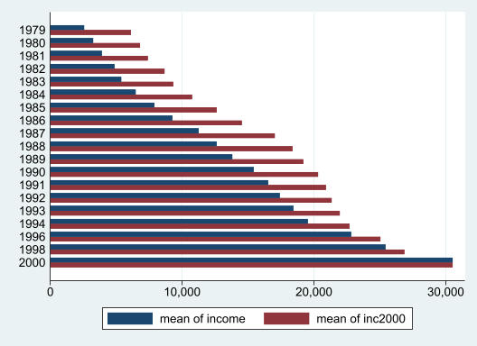
This will show you the mean income in each year, both in the original dollars and in 2000 dollars. Note how a dollar in 1979 was worth more than twice what a dollar was worth in 2000, but the difference decreases until in 2000 income and income2000 are identical.
6.7 Dealing with Duplicate Identifiers
The bane of everyone who does merges is the error message “variable id does not uniquely identify observations in the master data” and its variations. Sometimes this means you made a simple mistake: mixing up 1:m and m:1, for example, or specifying just one identifier when you need two. Sometimes it means you’ve badly misunderstood the structure of the data and need to rethink everything. But often it means there is a problem with the data itself: duplicate IDs.
If you follow the steps we recommend in First Steps with your Data, you’ll find out about any duplicates in the process of finding the data set’s identifiers (you’ll also avoid badly misunderstanding the structure of the data). However, it’s when you merge that duplicates become a problem that must be resolved. Fortunately, you now have the skills to resolve them.
The one thing you should not do is make the error message go away by changing the the type of merge you perform. If your merge should be one-to-one but you have duplicate identifiers in the master data set, changing it to many-to-one may allow the merge to run but the resulting data set won’t make any sense. If you find yourself wanting to run a many-to-many merge (m:m), step away from the computer, take a break, and then rethink what you’re doing. We’ve never seen a many-to-many merge that wasn’t a mistake; it’s hard to think of anything in the real world that could be modeled by what Stata does when you specify a many-to-many merge. Even the Stata documentation describes them as “a bad idea.”
The data sets we’ve been working with are carefully curated and will probably never have a duplicate identifier. However, they’re very common in administrative and other real-world data. So we’ve prepared a data set that does have some: merge_error.dta. This is a fictitious data set of students, their demographics, and their scores on a standardized test. Assume you were trying to merge it with another similar data set and got the dreaded “variable id does not uniquely identify observations in the master data.”
The first thing to do is load the data set that’s causing the error:
clear
use merge_error
describe
. clear

. use merge_error

. describe

Contains data from merge_error.dta
 Observations:           103
    Variables:             5                  1 Oct 2015 09:36
-------------------------------------------------------------------------------
Variable      Storage   Display    Value
    name         type    format    label      Variable label
-------------------------------------------------------------------------------
id              float   %9.0g
female          float   %9.0g
grade           int     %8.0g
race            int     %8.0g
score           int     %8.0g
-------------------------------------------------------------------------------
Sorted by:

.
The id variable is clearly intended to be an identifier, but recall that you can use duplicates report to check if it actually uniquely identifies observations:
duplicates report id
Duplicates in terms of id

--------------------------------------
   Copies | Observations       Surplus
----------+---------------------------
        1 |           91             0
        2 |           12             6
--------------------------------------
It does not–or you would not have gotten that error message–but this does not help us identify the problem. To do that, create a variable that tells you how many times each id is duplicated:
bysort id: gen copies = _NNow you can examine the problem observations with browse or list:
list if copies>1
     +---------------------------------------------+
     | id   female   grade   race   score   copies |
     |---------------------------------------------|
  9. |  9        1      11      0      76        2 |
 10. |  9        1      11      0      76        2 |
 27. | 26        1      11      0      85        2 |
 28. | 26        1      11      0      85        2 |
 35. | 33        0       8      0      78        2 |
     |---------------------------------------------|
 36. | 33        0       8      0      78        2 |
 67. | 64        0      10      1      86        2 |
 68. | 64        0      10      0      85        2 |
 77. | 74        0      11      0      63        2 |
 78. | 74        0       9      1      87        2 |
     |---------------------------------------------|
 97. | 94        1      11      1     100        2 |
 98. | 94        0      11      3     100        2 |
     +---------------------------------------------+
The first six rows consist of three pairs of observations which are completely identical. This is almost certainly a case of them having been put in the data set twice, a common data entry error. You can get rid of these duplicates by running:
duplicates drop
Duplicates in terms of all variables

(3 observations deleted)
This is a good outcome: not only is the problem easy to fix, you didn’t actually lose any data. Unfortunately it does not fix all the duplicates in this data set.
At this point copies is no longer accurate: it is still 2 for the observations where we dropped a duplicate observation. Update it before proceeding:
by id: replace copies = _N
list if copies>1
. by id: replace copies = _N
(0 real changes made)

. list if copies>1

     +---------------------------------------------+
     | id   female   grade   race   score   copies |
     |---------------------------------------------|
 64. | 64        0      10      1      86        2 |
 65. | 64        0      10      0      85        2 |
 74. | 74        0      11      0      63        2 |
 75. | 74        0       9      1      87        2 |
 94. | 94        1      11      1     100        2 |
     |---------------------------------------------|
 95. | 94        0      11      3     100        2 |
     +---------------------------------------------+

.
The remaining six rows with copies>1 are three pairs of observations with the same value of id but different values for one or more of the other variables. You should consider the possibility that there is some hierarchy involved that you were not aware of, such as some people taking multiple tests. However, there’s no indication of anything like that in this data set, and it would be unusual for it to affect so few observations. Almost certainly the duplicates are different people who were somehow given the same id, most likely due to a data entry error.
This is a bad outcome: Assuming you only have one person with an id of 64 in the other data set, you don’t know which of the two people with an id of 64 in this data set is the same person. You can resolve this problem by dropping both of the duplicate observations:
drop if copies>1(6 observations deleted)However, note that all of the duplicate observations have different values for race. This means that if you merged by id and race, they would be uniquely identified. This very much depends on the particulars of the data set: merging by id and female instead wouldn’t help much at all. On the other hand, if you had enough variables you might be able to match people even if the data sets didn’t have an identifier in common. Linking records without relying on identifiers is a very hot topic, but one we won’t address any further.
Exercise 4
nlsy_error.dta is a version of our NLSY extract that has had duplicate identifiers introduced into it. Identify and address the errors so that the combination of id and year are a unique identifier again and could be used to carry out a one-to-one merge.