In this chapter we’ll discuss variable transformations: creating and changing variables. You should already be familiar with the basics of variable transformations–if you’re not, Introduction to Stata: Creating and Changing Variables will get you up to speed. This chapter will add to your “bag of tricks” for working with numeric data.
4.1 Setting Up
Start a do file called numeric_transforms.do that loads acs.dta.
-------------------------------------------------------------------------------
      name:  <unnamed>
       log:  /home/r/rdimond/kb/dws/transforms.log
  log type:  text
 opened on:   2 Oct 2025, 17:14:45
4.2 Transformations and Missing Data
If an observation has a missing value for a variable, it should usually, but not always, have a missing value for any transformations of that variable.
Arithmetic operators (addition, subtraction, etc.) do this automatically. For example, to correct the incomes in this year 2000 ACS data set for inflation, we can convert them to (January) 2023 dollars by multiplying them by 1.77. But look at the result for household 484:
gen income_2023 = income * 1.77list household person age income income_2023 if household==484, ab(30)
The two children in the household have missing values for income, so they automatically got a missing value for income_2023. This is almost always what you want.
However, egen functions behave differently. In general, they act on the observed data and ignore the missing data. For example, consider calcualting household incomes using the egentotal function (and by):
by household: egen household_income = total(income)list household person age income household_income if household==484, ab(30)
The total function added up all the observed values of income and ignored the missing values. This had the effect of treating the missing values as zeros, but that isn’t a general rule. The mean function will calculate the mean of the observed values, which has the effect of treating missing values as if they were at the mean. Be sure to think through whether the behavior of egen makes sense for your particular task.
Conditions never return a missing value, even if they involve missing values. For example, consider creating an indicator for high_income with the threshold for high being $50,000:
gen high_income_oops = (income > 50000)list household person age income high_income_oops if household==484, ab(30)
Recall that the way Stata handles missing values is to designate the 27 largest possible values of each variable type as the various flavors of missing (., .a, .b, .c, up though .z). But when it comes to conditions (unlike arithmatic operators or egen functions) missing values are just treated like the big numbers they really are. Thus the following inequalities hold:
Missing Values and Inequalities
Any observed value or normal number < . < .a < .b < .c … < .x < .y < .z
That’s why the children, with their missing values for income got a 1 for high_income: to Stata . is biggger than 50000 or any other number.
The solution is to exclude observations with missing values from the process of creating the new variable entirely. Thus they’ll be left with a missing value, which is what you want.
gen high_income= (income > 50000) if income < .list household person age income high_income if household==484, ab(30)
Why income < . rather than income != .? Because income < . excludes all the missing values (., .a, .b, etc.), not just ..
However, subtle differences in what you want your variable to mean can change how you handle missing values. Suppose you wanted an indicator for “this person is known to have a high income.” Now anyone with a missing value for income should have a 0 for the new indicator because they are not known to have a high income. But you can’t just ignore the missing values, or people with a missing value will get a 1. Instead, a person should get a 1 for known_high_income if their income is both high and known:
gen known_high_income = (income > 50000) & (income < .)list household person age income known_high_income if household==484, ab(30)
4.3 Conditional Transformations (Transformations that Vary for Subsets)
Often a variable transformation must be different for different subsets of the data. As a trivial example, suppose you wanted to define an education score for each person which is:
25 if they do not have a bachelor’s degree
75 if they do have a bachelor’s degree or higher
We’ll explore several ways of creating this ed_score variable.
First off, let’s remind ourselves how edu is defined so we can figure out how to identify people with bachelor’s degrees or higher. Run describe edu to get the name of the value labels associated with it:
describe edu
Variable      Storage   Display    Value
    name         type    format    label      Variable label
-------------------------------------------------------------------------------
edu             byte    %24.0g     edu_label
                                              Educational Attainment
Next use label list edu_label to see what the labels mean:
labellist edu_label
edu_label:
           0 Not in universe
           1 None
           2 Nursery school-4th grade
           3 5th-6th grade
           4 7th-8th grade
           5 9th grade
           6 10th grade
           7 11th grade
           8 12th grade, no diploma
           9 High School graduate
          10 Some college, <1 year
          11 Some college, >=1 year
          12 Associate degree
          13 Bachelor's degree
          14 Master's degree
          15 Professional degree
          16 Doctorate degree
The presence of the “Not in universe” label is a good reminder that the Census Bureau did not collect education data for people under the age of three, so we set those values to missing. But let’s assume that no one under the age of three can possibly have a bachelor’s degree.
The values 13, 14, 15, and 16 indicate a bachelor’s degree or higher, or, to put it more succinctly, edu>=13. But remember that Stata considers missing to be greater than 13, and we want to assume that missing means no bachelor’s degree. Thus the complete condition for identifying people with a bachelor’s degree is (edu >= 13) & (edu < .).
Since we’ll use need to identify people with a bachelor’s degree condition multiple times, it will be convenient to create an indicator variable for it so we don’t have to type out the full condition every time:
gen bachelors = (edu >= 13) & (edu < .)
The straightforward way to create ed_score is two commands that essentially translate the original definition into Stata:
gen ed_score = 25 if !bachelorsreplace ed_score = 75 if bachelorslist household person edu ed_score in 1/5
(4,485 missing values generated)
(4,485 real changes made)

     +-------------------------------------------------------+
     | househ~d   person                      edu   ed_score |
     |-------------------------------------------------------|
  1. |       37        1   Some college, >=1 year         25 |
  2. |       37        2   Some college, >=1 year         25 |
  3. |       37        3   Some college, >=1 year         25 |
  4. |      241        1          Master's degree         75 |
  5. |      242        1        Bachelor's degree         75 |
     +-------------------------------------------------------+
That works just fine for this simple example. But if this were just part of a more complex calculation it would be useful to have a single mathematical expression that can calculate both values. You can do that using the cond() function. The cond() function takes three arguments:
A condition
The result if the condition is true
The result if the condition is false
In this case, the first argument could be either (edu >= 13) & (edu < .) or just the indicator variable bachelors. If that is true, then the person has a bachelor’s degree or higher and the education score should be 75, so 75 is the second argument. If that is false, the person does not have a bachelor’s degree and education score should be 25, so 25 is the third argument.
gen ed_score2 = cond(bachelors, 75, 25)list household person edu ed_score2 in 1/5
     +-------------------------------------------------------+
     | househ~d   person                      edu   ed_sco~2 |
     |-------------------------------------------------------|
  1. |       37        1   Some college, >=1 year         25 |
  2. |       37        2   Some college, >=1 year         25 |
  3. |       37        3   Some college, >=1 year         25 |
  4. |      241        1          Master's degree         75 |
  5. |      242        1        Bachelor's degree         75 |
     +-------------------------------------------------------+
An alternative way of looking at this notes that you can think of the original definition of education score as saying that everyone starts with an education score of 25 points, and then people with a bachelor’s degree or higher get an additional 50 points. That can be implemented with:
gen ed_score3 = 25replace ed_score3 = ed_score3 + 50 if bachelorslist household person edu ed_score3 in 1/5
(4,485 real changes made)

     +-------------------------------------------------------+
     | househ~d   person                      edu   ed_sco~3 |
     |-------------------------------------------------------|
  1. |       37        1   Some college, >=1 year         25 |
  2. |       37        2   Some college, >=1 year         25 |
  3. |       37        3   Some college, >=1 year         25 |
  4. |      241        1          Master's degree         75 |
  5. |      242        1        Bachelor's degree         75 |
     +-------------------------------------------------------+
Setting a variable equal to itself plus something is a very common and useful pattern.
Now consider this alternative:
gen ed_score4 = 25 + 50*bachelorslist household person edu ed_score4 in 1/5
     +-------------------------------------------------------+
     | househ~d   person                      edu   ed_sco~4 |
     |-------------------------------------------------------|
  1. |       37        1   Some college, >=1 year         25 |
  2. |       37        2   Some college, >=1 year         25 |
  3. |       37        3   Some college, >=1 year         25 |
  4. |      241        1          Master's degree         75 |
  5. |      242        1        Bachelor's degree         75 |
     +-------------------------------------------------------+
bachelors is either 1 or 0. For people without a bachelor’s degree it is 0, so 50 multiplied by 0 goes away and they just get the original 25. For people with a bachelor’s degree it is 1, so 50 is multiplied by 1 and they get a total of 75.
This is exactly how indicator variables work in regression models. If this were a regression model, 50 would be the coefficient on the covariate bachelors and the predicted value would be either 25 or 75. Interaction terms are very similar. If 50 were the coefficient on an interaction between bachelors and age, then it would be 50 * bachelors * age, and again the entire term disappears (is multiplied by 0) for people who do not have a bachelor’s degree. It becomes just 50*age for people who do.
All of these could be done using the original condition (edu>=13) & (edu<.) rather than the indicator bachelors, even the last version.
gen ed_score5 = 25 + 50*((edu>=13) & (edu<.))list household person edu ed_score5 in 1/5
     +-------------------------------------------------------+
     | househ~d   person                      edu   ed_sco~5 |
     |-------------------------------------------------------|
  1. |       37        1   Some college, >=1 year         25 |
  2. |       37        2   Some college, >=1 year         25 |
  3. |       37        3   Some college, >=1 year         25 |
  4. |      241        1          Master's degree         75 |
  5. |      242        1        Bachelor's degree         75 |
     +-------------------------------------------------------+
When a condition appears in a mathematical expression, Stata automatically recognizes it, the result is either 0 or 1, and that is used in evaluating the rest.
4.4 Conditions with Many Values
The values of edu that mean “bachelor’s degree or higher” are 13, 14, 15, and 16. It’s highly convenient to specify them using the inequalities (edu >= 13) & (edu < .) and by all means you should do that where possible. But sometimes the values you need don’t match a simple pattern and you need to list them all. You could specify them with a series of conditions combined with logical or:
(edu==13) | (edu==14) | (edu==15) | (edu==16)
You’re probably thinking “Surely there’s an easier way” and there is: the inlist() function. The first argument of inlist() is a variable, and the rest are possible values of that variable. The result is 1 (true) if the actual value of the variable is in the list, and 0 (false) if it is not. Use it wherever you would use a condition, including inside mathematical expressions:
gen bachelors2 = inlist(edu, 13, 14, 15, 16)gen ed_score6 = 25 + 50*inlist(edu, 13, 14, 15, 16)list household person edu bachelors2 ed_score6 in 1/5
     +------------------------------------------------------------------+
     | househ~d   person                      edu   bachel~2   ed_sco~6 |
     |------------------------------------------------------------------|
  1. |       37        1   Some college, >=1 year          0         25 |
  2. |       37        2   Some college, >=1 year          0         25 |
  3. |       37        3   Some college, >=1 year          0         25 |
  4. |      241        1          Master's degree          1         75 |
  5. |      242        1        Bachelor's degree          1         75 |
     +------------------------------------------------------------------+
Note that you can also use inlist() with a string variable, in which case the values must be strings.
The related inrange() function takes three arguments: a variable, and the beginning and end of a range. It returns 1 if the variable is in the range specified and 0 otherwise.
gen bachelors3 = inrange(edu, 13, 16)list household person edu bachelors3 in 1/5
     +-------------------------------------------------------+
     | househ~d   person                      edu   bachel~3 |
     |-------------------------------------------------------|
  1. |       37        1   Some college, >=1 year          0 |
  2. |       37        2   Some college, >=1 year          0 |
  3. |       37        3   Some college, >=1 year          0 |
  4. |      241        1          Master's degree          1 |
  5. |      242        1        Bachelor's degree          1 |
     +-------------------------------------------------------+
4.5 Creating Quantiles
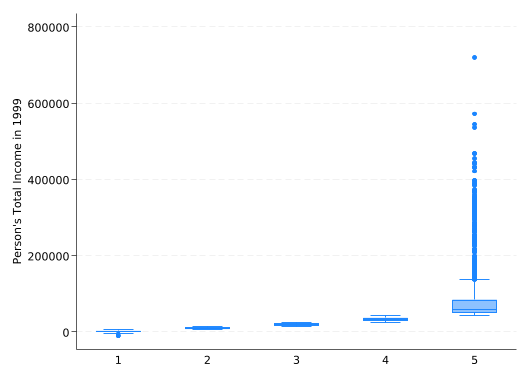
Dividing a data set into quantiles is a very common task, and is easily carried out using the xtile command. For example, you can assign the adults in the ACS to their income quintile with:
xtile inc_quint = income if age>=18, n(5)
The n() option specifies the number of quantiles.
The result will be an ordered categorical variable, frequently used for grouping with the by prefix or with over() in graphs. For example, you can create a box plot of income over the five quintiles with:
graph box income, over(inc_quint)
4.6 Creating Categorical Variables From Cutpoints
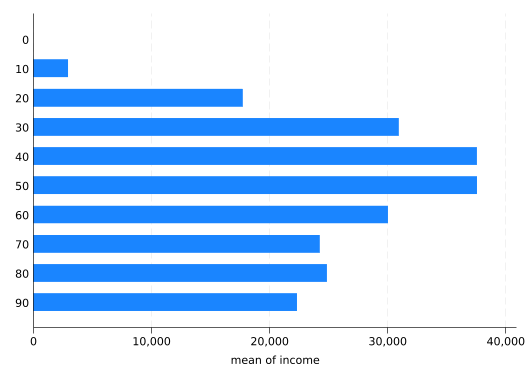
An alternative way to use xtile is to define a categorical variable based on a continuous variable with cutpoints that define the categories. As an example, we’ll use it to categorize age by decade (20s, 30s, etc.).
The cutpoints must be put in a variable in the data set, normally one you’ll create just for this purpose. But the values won’t actually belong to the observations they’re attached to. Rather the value of the cutpoint for the first observation will be the maximum value for the first category, the value for the second observation will be the maximum for the second category, etc. The maximum value is included in the category (i.e. the rule is value <= max). You should have more observations than categories, so the rest will get missing values. Normally you’ll drop this variable as soon as you’re done with it.
For decades we want the cutpoints to be 9, 19, 29 up through 99 (recall that in the ACS 93 really means “93 or older”). You can do that with:
gen cutpoints = _n*10 - 1 if_n<=10list cutpoint in 1/12, ab(30)
You can set completely arbitrary cutpoints if you need to. This is one of the few places where you might use in for actual work. For example, if you wanted your first category to be everyone below 18 and your second to be everyone between 18 and 30, you could do:
gen cutpoints = 18 in 1
replace cutpoints = 30 in 2
Having defined your cutpoints, you can now run xtile with the cut() option, which tells it to use cutpoints instead of quantiles and gives the name of the variable that contains the cutpoints.
xtile decade = age, cut(cutpoints)list age decade in 1/5
The categories seem off because they are numbered starting with 1, so right now a 1 for decade means ages 0-9, 2 means ages 10-19, etc. While the values of a categorical variable are completely arbitrary in theory, if you subtract 1 and then multiply by 10, 0-9 will be 0, 10-19 will be 10, 20-29 will be 20, etc. and that’s a good bit more intuitive.
replace decade = (decade - 1)*10list age decade in 1/5
Now it’s ready for use, for example plotting the mean income by decade:
graphhbar income, over(decade)
4.7 Extracting Digits From Numbers
You may be thinking “That’s nice, but couldn’t we have gotten decade by just dividing age by 10?” Almost: you want to divide by ten and get rid of the fractional part. You can do that by telling Stata that the new variable you’re creating should be an integer:
Stata will do the division normally but, because the decade2 variable is an integer, when it comes time to store the result any fractional part is discaded. Thus if age/10 is 19, only the 1 is stored. This integer division is surprisingly useful.
Note that this time ages 0-9 are decade 0, but you probably still want to multiply by 10 so 20-29 is 20 instead of 2.
replace decade2 = decade * 10list age decade in 1/5
If you wanted just the last digit of age, you could get that with the mod() (modulus) function. It takes two arguments and returns the remainder when the first is divided by the second:
The combination of integer division and modulus allows you to split numbers up at will. For example, the FIPS code for Dane County, Wisconsin is 55025, where 55 is the code for Wisconsin. But if you want to do analysis at the state and county level, you may need separate state and county variables. You can do that with:
gen fips = 55025genint state = fips/1000gen county = mod(fips, 1000)list fips state county in 1
     +------------------------+
     |  fips   state   county |
     |------------------------|
  1. | 55025      55       25 |
     +------------------------+
(Note that for many purposes you can use state and the original FIPS code, as the original code unqiquely identifies counties.)
The county variable does not include a leading zero–numeric variables never do. Most of the time that’s not a problem: FIPS codes do not use 25 and 025 to mean different counties. You can tell Stata to print a numeric variable with leading zeros. But if you really need 25 and 025 to mean different things store the variable as a string.
::{.callout-note} ### Exercise
Given the telephone number 6082629917, extract the area code. Then extract the last four digits. :::
4.8 Rounding
You might be tempted to think of the integer division gen int state = fips/1000 as “rounding to the nearest 1000”, but it’s actually quite different from rounding. You’ll see why if you try to generate decade by rounding to the nearest 10. The round() function takes two arguments: the number to be rounded and the second the number to round to.
gen decade3 = round(age, 10)list age decade3 in 1/5
Integer division set decade2 to 1 for observation 2: dividing 19 by 10 gives 1.9, but the .9 is discarded. Rounding (decade3) rounded observation 2’s age up to 20. Which one is right depends on what you’re trying to do.