When you start work with a data set, your first goals are to understand the data set and to clean it up. Logically these are two separate processes, but in practice they are intertwined: you can’t clean your data set until you understand it at some level, but you won’t fully understand it until it’s clean. Thus this chapter will cover both.
I’ll also introduce some data science concepts in this chapter. This makes for lengthy discussions of tasks that in practice you can complete very quickly.
In this chapter, we’ll primarily use the file 2000_acs_sample.dta. This file started as the 1% unweighted sample of the 2000 American Community Survey available from IPUMS, but then I took a 1% random sample of the households in that dataset just to make it easier to work with. This data set uses the “source” variables directly from the Census Bureau rather than the “harmonized” variables created by IPUMS, which are much cleaner. For real work you can usually use the harmonized variables, but we’re here to learn how to do the kinds of things IPUMS does to create them.
By using this data set in the examples, you’ll also gain some basic understanding of the U.S. population (as of 2000) and some experience with a real and important data set, but you would not want to use this particular data file for research. For that, go get the original data from IPUMS.
Setting Up
Start a do file that loads 2000_acs_sample.dta, and make it a proper do file (i.e. it keeps a log, starts with a blank slate, etc.). Call it first_steps_examples.do.
The following version loads the dataset from the web. If you downloaded the example files, your use command can be just use 2000_acs_sample.
-------------------------------------------------------------------------------
      name:  <unnamed>
       log:  /home/d/dimond/kb/dws/first_steps_examples.log
  log type:  text
 opened on:  24 Nov 2025, 17:16:47
3.1 Read the Documentation
When you download a data set, you’ll be tempted to open it up and go to work right away. Resist! Time spent reading the data set’s documentation (assuming there is some) can save you much more time down the road. Data providers may give you files containing documentation along with the data itself, or it may be on their web site. Feel free to skim what’s not relevant to you–this chapter will give you a better sense of what information is most important.
Unfortunately, not all data sets have good documentation, or any documentation at all, so figuring out the nature of a data set by looking at the data set itself is a vital skill. You also can’t assume that the documentation is completely accurate, so you need to check what it says.
The ACS has lots of good documentation, but for practice we’ll make minimal use of it (just the codebook) and figure out everything we can for ourselves. We’d still do all the same things if we were using the documentation, we’d just understand what we were looking at much more quickly.
3.2 Identify the Variables
The describe command will give you basic but useful information about your data set:
describe
Contains data from https://sscc.wisc.edu/sscc/pubs/dws/data/2000_acs_sample.dta
 Observations:        28,172
    Variables:            16                  8 Apr 2019 16:43
-------------------------------------------------------------------------------
Variable      Storage   Display    Value
    name         type    format    label      Variable label
-------------------------------------------------------------------------------
year            int     %8.0g      year_lbl   Census year
datanum         byte    %8.0g                 Data set number
serial          double  %8.0g                 Household serial number
hhwt            double  %10.2f                Household weight
gq              byte    %43.0g     gq_lbl     Group quarters status
us2000c_seria~o str7    %9s                   Housing/Group Quarters (GQ) Unit
                                                Serial Number
pernum          int     %8.0g                 Person number in sample unit
perwt           double  %10.2f                Person weight
us2000c_pnum    str2    %9s                   Person Sequence Number
us2000c_sex     str1    %9s                   Sex
us2000c_age     str2    %9s                   Age (original)
us2000c_hispan  str2    %9s                   Hispanic or Latino Origin
us2000c_race1   str1    %9s                   Race Recode 1
us2000c_marstat str1    %9s                   Marital Status
us2000c_educ    str2    %9s                   Educational Attainment
us2000c_inctot  str7    %9s                   Person's Total Income in 1999
-------------------------------------------------------------------------------
Sorted by: serial  pernum
The primary goal of running describe is to see what variables you have and what they’re called. The variable labels will help you understand what they mean.
You’ll also want to start a “to do list” of issues you need to address before analyzing the data. Here are some issues brought out by running describe on this data set:
The data set seems to have an excess of identifiers: serial and serialno, pernum and us2000c_pnum.
Since you’re using a single data set from a single year, you probably don’t need year and datanum to tell you where each observation comes from.
For the same reason, you also don’t need us2000c_ (US 2000 Census) in your variable names to tell you where the variables came from.
You have both household weight (hhwt) and person weight (pwt) variables even though this is supposed to be an unweighted sample.
pnum, and all of the us2000c_ variables are stored as strings of various lengths, even though some of them are clearly intended to be numeric variables.
Another issue to watch out for is the storage type of identifier variables. The default variable type, float, has seven digits of accuracy. Identifiers that are more than seven digits long must be stored as double (numbers with 16 digits of accuracy), as long (integers with up to 10 digits), or as strings (text with up to a billion characters). In this data set serial is stored as double and us2000c_pnum as string, so those are fine. The pernum variable, on the other hand, is an int (integer), so it can only have five digits. (This is our first hint that pernum by itself is not a unique identifier.)
Note which variables have value labels: with those variables, what you see in output will be the labels and not the underlying values. You need to use the values in your code. You can see what all the underlying values are with label list but it’s long, especially since this data set makes the interesting choice of applying value labels to year which are identical to the values themselves. (Most likely there are some circumstances where they apply a different label.) You can also list a single label using the label names you get from describe:
labellist gq_lbl
gq_lbl:
           0 Vacant unit
           1 Households under 1970 definition
           2 Additional households under 1990 definition
           3 Group quarters--Institutions
           4 Other group quarters
           5 Additional households under 2000 definition
           6 Fragment
This is a more typical set of value labels. Looking at this definition tells you that if you wanted to limit your analysis to “Households under 1970 definition” the code for that restriction would be if gq==1.
3.3 Look at the Data
Unless your data set is very small, you can’t practically read all of it. But just looking at a few rows may allow you to immediately spot patterns that would be difficult to detect using code. In this case, opening the data browser (type browse or click the button that looks like a magnifying glass over a spreadsheet) will show the following:
year and datanum seem to always have the same value, suggesting that we don’t need them.
hhwt and perwt (household and person weights) seem to always be 100.00, which makes sense given that this is supposed to be an unweighted sample.
pernum and us2000c_pnum appear to be identical other than us2000c_pnum being a string and having leading zeros.
pernum seems to count observations, starting over from 1 every time serial changes.
All of the string variables contain mostly numbers.
us2000c_sex, us2000c_hispan, us2000c_race1, and us2000c_marstat are clearly describing categories, but even though they are string variables they only contain numbers. We will have to refer to the codebook to find out what the numbers mean. (This also applies to us2000c_educ, it’s just not as obvious at this point.)
us2000c_inctot sometimes has “BBBBBBB”, which is certainly an odd value for income.
You can’t be sure that these patterns hold the for entire data set until you check, but now you know some things to check for. For example, you can tab to confirm that year and datanum always contain the same value:
tabyear
Census year |      Freq.     Percent        Cum.
------------+-----------------------------------
       2000 |     28,172      100.00      100.00
------------+-----------------------------------
      Total |     28,172      100.00
tab datanum
   Data set |
     number |      Freq.     Percent        Cum.
------------+-----------------------------------
          4 |     28,172      100.00      100.00
------------+-----------------------------------
      Total |     28,172      100.00
Exercise
Load the dataset 2000_acs_sample_harm.dta (or https://sscc.wisc.edu/sscc/pubs/dws/data/2000_acs_sample_harm.dta). This is a similar sample but with the IPUMS “harmonized” variables. Run describe, run label list for a few variables, and look at it in the data browser. What do you notice? What issues did IPUMS resolve? What issues remain?
When you’re done be sure to load 2000_acs_sample again.
Contains data from https://sscc.wisc.edu/sscc/pubs/dws/data/2000_acs_sample_har
> m.dta
 Observations:        28,085
    Variables:            18                  19 Mar 2019 13:50
-------------------------------------------------------------------------------
Variable      Storage   Display    Value
    name         type    format    label      Variable label
-------------------------------------------------------------------------------
year            int     %8.0g      year_lbl   Census year
datanum         byte    %8.0g                 Data set number
serial          double  %8.0g                 Household serial number
hhwt            double  %10.2f                Household weight
gq              byte    %43.0g     gq_lbl     Group quarters status
pernum          int     %8.0g                 Person number in sample unit
perwt           double  %10.2f                Person weight
sex             byte    %8.0g      sex_lbl    Sex
age             int     %36.0g     age_lbl    Age
marst           byte    %23.0g     marst_lbl
                                              Marital status
race            byte    %32.0g     race_lbl   Race [general version]
raced           int     %182.0g    raced_lbl
                                              Race [detailed version]
hispan          byte    %12.0g     hispan_lbl
                                              Hispanic origin [general version]
hispand         int     %24.0g     hispand_lbl
                                              Hispanic origin [detailed
                                                version]
educ            byte    %25.0g     educ_lbl   Educational attainment [general
                                                version]
educd           int     %46.0g     educd_lbl
                                              Educational attainment [detailed
                                                version]
inctot          long    %12.0g                Total personal income
ftotinc         long    %12.0g                Total family income
-------------------------------------------------------------------------------
Sorted by:
labellist sex_lbl race_lbl
sex_lbl:
           1 Male
           2 Female
race_lbl:
           1 White
           2 Black/African American/Negro
           3 American Indian or Alaska Native
           4 Chinese
           5 Japanese
           6 Other Asian or Pacific Islander
           7 Other race, nec
           8 Two major races
           9 Three or more major races
The variable names have been cleaned up, and many variables that are strings containing numbers in the source data are have been converted to numbers with value labels in the harmonized data. Much more useful!
The year and datanum variables are still there, and still don’t look useful to us. Also, hhwt and perwt are still there, and still seem to be always 100.
This data set includes “detailed version” of the race and hispanic variables. (If you list their value labels, you’ll see they’re very detailed indeed.) They aren’t a result of wrangling the source data, they’re just included in the harmonized data set by default.
Looking in the data browser, you’ll notice a lot of rows have the value 9999999 for inctot (total income). It’s quite a coincidence that so many people made exactly nine million, nine hundred ninety-nine thousand, nine hundred ninety-nine dollars in the last year. It’s especially remarkable once you realize they’re all children! In reality, 9999999 is a code for missing. That’s described in the data documentation, but one way or another it’s critical that you notice and correct such things. If you tried to do any analysis using inctot right now, Stata would treat 9999999 as a valid value and you would get wildly inaccurate results. We’ll cover recoding missing values later, once we have more tools for detecting them.
3.4 Find the Identifiers and Figure Out the Data Structure
Imagine you wanted to call someone’s attention to a particular value in this data set. How could you tell them exactly which row and column to look at?
3.4.1 Observation Numbers
One way to tell them which row to look at is to simply tell them the observation number. Observation numbers are tracked by the system variable _n, which you can use in commands as if it were any other variable. If you are using by the variable _n will take that into account, meaning it will start over from 1 in every by group. We’ll use that heavily later.
The trouble with observation numbers is that many common tasks change them: sorting, for example, or dropping or adding observations. Thus it’s far better to use one or more identifier variables. If the data set does not contain identifier variables, you can create one based on the current observation numbers with gen id = _n. Then the variable id will not change even if the observation numbers do.
3.4.2 Identifier Variables
Identifier variables, also known as primary keys or indexes, are variables whose purpose is to identify observations. They normally do not contain information. If you had a data set where each row was a UW-Madison student, their UW-Madison ID number would be a unique identifier: specifying a UW-Madison ID number allows you to identify a single row.
Now imagine a data set describing UW-Madison students, but there is one row for each class the student is currently taking, with each class being identified by a number. In order to identify a specific row you now need to specify both a UW-Madison ID number and a class number. The combination of ID number and class number would be a compound identifier for the data set, and the combination of the two is a unique identifier.
Finding the identifier variables in a data set will help you understand the structure of the data. If student ID is a unique identifier, you know you have one row per student and an observation represents a student. If student ID and class number are a unique identifier, you know you have one row per student per class, and each observation represents a class/student combination. In practice you might refer to an observation as a class, as long as everyone understands that two students taking the same class will be two rows, not one.
The duplicates report command can easily identify whether a variable or set of variables is a unique identifier: if it is, there will be no duplicates. The ACS data has a variable called pernum (Person number in sample unit) is it a unique identifier?
Clearly not: only four observations can be uniquely identified using pernum. Running tab on an identifier wouldn’t normally be useful because there will be too many values, but the large number of duplicates suggests it might be fruitful here:
Seeing the values, we can guess what this variable is: the person’s identifier within their household. So pernum is not an unique identifier by itself, but it is part of a compound identifier that is. Try:
duplicatesreport serial pernum
Duplicates in terms of serial pernum

--------------------------------------
   Copies | Observations       Surplus
----------+---------------------------
        1 |        28172             0
--------------------------------------
There are no duplicates so we now know that serial and pernum are a compound identifier for this data set. serial identifies a household and pernum identifies a person with in that household. We also know that each observation represents a person, and the people are grouped into households.
3.4.3 Column Identifiers
In Stata, columns are identified by variable names. Variable names are always unique (Stata won’t allow you to create two variables with the same name) but they often have multiple parts. In this data set, some of the variable names are in the form source_variable, like us2000c_sex and us2000c_age. It can be very useful to think of such variable names as a compound identifier with two separate parts (e.g. source and variable). It’s even possible to convert row identifiers to part of a compound column identifier and vice versa–we’ll learn how later.
3.4.4 Using Identifiers
Stata does not give identifiers any special status, so you use them like any other variable. If you want to see observation 5, run:
Another way to identify the value of a specific variable for a specific observation number is to put the observation number in square brackets after the variable name.
display us2000c_age[5]
29
This square bracket syntax can be used in mathematical expressions, which is very useful.
Note: while the list command lists your data, the display command prints out a single thing. This can be the result of evaluating a mathematical expression (display 2+2) or a message contained in quotes (display "Completed discussion of identifiers"), both of which can be quite useful.
Exercise 3
Load the data set atus.dta (or https://sscc.wisc.edu/sscc/pubs/dws/data/atus.dta). This is a selection from the American Time Use Survey, which measures how much time people spend on various activities. Find the identifiers in this data set. What does an observation represent? What was the first activity recorded for person 20170101170012?
Be sure to reload 2000_acs_sample when you’re done.
Solution
Load the data, then run describe to see what variables it contains.
Contains data from https://sscc.wisc.edu/sscc/pubs/dws/data/atus.dta
 Observations:       199,894
    Variables:            21                  11 Apr 2019 15:44
-------------------------------------------------------------------------------
Variable      Storage   Display    Value
    name         type    format    label      Variable label
-------------------------------------------------------------------------------
year            long    %12.0g                Survey year
caseid          double  %20.0f                ATUS Case ID
famincome       int     %20.0g     famincome_lbl
                                              Family income
pernum          byte    %8.0g      pernum_lbl
                                              Person number (general)
lineno          int     %21.0g     lineno_lbl
                                              Person line number
wt06            double  %17.0g                Person weight, 2006 methodology
age             int     %8.0g                 Age
sex             byte    %21.0g     sex_lbl    Sex
race            int     %42.0g     race_lbl   Race
hispan          int     %22.0g     hispan_lbl
                                              Hispanic origin
asian           int     %12.0g     asian_lbl
                                              Asian origin
marst           byte    %24.0g     marst_lbl
                                              Marital status
educ            int     %47.0g     educ_lbl   Highest level of school completed
educyrs         int     %36.0g     educyrs_lbl
                                              Years of education
empstat         byte    %22.0g     empstat_lbl
                                              Labor force status
fullpart        byte    %21.0g     fullpart_lbl
                                              Full time/part time employment
                                                status
uhrsworkt       int     %8.0g                 Hours usually worked per week
earnweek        double  %7.2f                 Weekly earnings
actline         byte    %8.0g                 Activity line number
activity        long    %73.0g     activity_lbl
                                              Activity
duration        int     %8.0g                 Duration of activity
-------------------------------------------------------------------------------
Sorted by:
To find the identifier(s), remember identifiers rarely contain information. That excludes most of the variables. caseid, pernum, lineno, and actline seem like good candidates. But if you look at the data in the data browser, you’ll see that pernum and lineno are always 1, so they’re out.
Next use duplicates report to figure out which candidate identifier or combination of candidate identifiers uniquely identify the observations.
Clearly caseid alone does not uniquely identify observations, which tells us this data set does not consist of one row per “case.” I’ll omit checking actline the same way, but it alone doesn’t uniquely identify observations either. How about the combination of caseid and actline?
duplicatesreport caseid actline
Duplicates in terms of caseid actline

--------------------------------------
   Copies | Observations       Surplus
----------+---------------------------
        1 |       199894             0
--------------------------------------
Bingo. A “case” here is a person, and actline or “activity line” identifies an activity. This is a time use survey, so it makes sense that we have one row per person per activity. Thus an observation represents an activity, as long as we understand that two people doing the same activity (or, it turns out, one person doing the same activity twice at two different times) is two observations.
To identify the first activity for person 20170101170012, we want the value of activity for the row where caseid is 20170101170012 and actline is 1:
list activity if caseid==20170101170012 & actline==1
Understanding data takes time. Even skipping past data you don’t care about to get to what you do care about takes time. So if you won’t use parts of a data set, get rid of those parts sooner rather than later. Doing so will also reduce the amount of memory needed to analyze your data and the amount of disk space needed to store it, and make anything you do with it run that much faster. If you change your mind about what you need, you can always change your do file later.
The drop command can remove either variables or observations from your data set, depending on whether it is followed by a variable list or an if condition. To drop year and datanum, run:
dropyear datanum
Let’s declare that you don’t want to include individuals living in “group quarters” (prisons, for example) in your analysis. Drop them with:
dropif gq==3 | gq==4
(762 observations deleted)
The keep command works in the same way, but in the opposite sense: running keep year datanum would drop all the variables except year and datanum. Running keep if gq==3 | gq==4 would drop everyone except those in group quarters. If you start with a data set that contains thousands of variables but only intend to use a dozen (very common), a keep command that cuts the data set down to just that dozen is an excellent starting point. On the other hand, if those variables have names that are codes rather than anything meaningful (also very typical in large data sets), consider renaming them first so you only have to use the ugly codes once.
3.6 Change Variable Names
A good variable name tells you clearly what the variable contains. Good variable names make your code easier to understand, easier to debug, and easier to write. If you have to choose between making a variable name short and making it clear, go with clear.
When you use abbreviations use the same abbreviation every time, even across projects. This data set abbreviates education as educ, and there’s nothing wrong with that, but I use edu in my other projects and that’s sufficient reason to change it.
Variable names cannot contains spaces, but many variable names should contain multiple words. I suggest you use underscores (_) as a substitute for spaces, as in household_income. This is known as snake case because the underscore looks like a snake crawling on the ground. The main alternative is householdIncome, known as camel case. I find camel case harder to read, but I don’t really care which you use as long as you’re consistent. Don’t make yourself try to remember every time if you used household_income or householdIncome for the project you’re working on! Just combining words without any indication of where the second word begins, like householdincome, is right out.
The syntax to change a single variable name is just rename old_name new_name. Change pernum to person with:
rename pernum person
The rename command can rename groups of variables as well. We’re not planning to combine our example data with other data sets, so we don’t need the us2000c_ at the beginning of many of the variable names to tell us which data set the variable came from. You can remove it with:
rename us2000c_* *
This can be read as “rename all the variables that match the pattern us2000c_ followed by something to just the something.” Type help rename group to see the various ways you can rename groups of variables.
Many of the resulting variable names are easy to remember once you know what they are but cryptic on a first reading. We’ll make them clearer in the exercise.
Exercise
Rename race1 to race, serial to household, educ to edu, hispan to hispanic, marstat to marital_status, and inctot to income.
Note that we will use these new variable names from now on. Even if you don’t do the exercise yourself, run the code from the solution if you’re coding along with the discussion (as you should be!). That will be true for all the remaining exercises.
Solution
rename race1 racerename serial householdrename educ edurename hispan hispanicrename marstat marital_statusrename inctot income
3.7 Convert String Variables that Contain Numbers to Numeric Variables
Unfortunately, it’s very common for numeric variables to be imported into Stata as strings. Before you can do much work with them they need to be converted into numeric variables.
The destring command is the easy way to convert strings to numbers. Just give it a varlist to act on, and the replace option to tell it it can replace the existing string variables with the new numeric versions. You have some of these in the ACS sample; destring the ones you’re interested in with:
destring sex age hispanic race marital_status edu income, replace
sex: all characters numeric; replaced as byte
age: all characters numeric; replaced as byte
hispanic: all characters numeric; replaced as byte
race: all characters numeric; replaced as byte
marital_status: all characters numeric; replaced as byte
edu: all characters numeric; replaced as byte
income: contains nonnumeric characters; no replace
Before carrying out a conversion, Stata checks that all the string variable’s values can be successfully converted to numbers. In the case of income, Stata found that some values could not be. Technically this is not an error (your do file did not crash) but income was not converted. To explore why, use the gen() option to create a new variable containing the numeric values, and the force option to tell Stata to proceed with the conversion despite the values that cannot be converted.
destring income, gen(income_test) force
income: contains nonnumeric characters; income_test generated as long
(6144 missing values generated)
The force option is so named because you’re forcing Stata to do something it doesn’t think is a good idea. This should make you nervous! Only use a force option if you’re very confident that you understand both why Stata thinks what you’re doing might be a bad idea and why it’s okay in your case.
With both income (the original string variable) and income_test (the new numeric version) available to you, you can compare them and figure out what’s going on. Observations with values of income that could not be converted have missing values for income_test, so get a list of the values of income that could not be converted with tab:
tab income if income_test==.
   Person's |
      Total |
  Income in |
       1999 |      Freq.     Percent        Cum.
------------+-----------------------------------
    BBBBBBB |      6,144      100.00      100.00
------------+-----------------------------------
      Total |      6,144      100.00
There’s only one value that couldn’t be converted, “BBBBBBB”. This is a code for missing, so it should be converted to a missing value: destring did exactly what you want it to do. Now that you know that, you can go back and just convert income using the force option rather than creating a separate income_test variable. But you want to keep a record that you checked and know that that’s okay to do.
Go back in your do file and comment out (i.e. turn into comments) both the destring command that created income2 and the tab command that checked it against income. Add text that explains what you found and why that means you don’t have to worry about the values that cannot be converted. Then add the force option to your original destring command. Rerun your do file so that the data set no longer contains income_test and income is numeric. The result might look like this:
destring sex age hispanic race marital_status edu income, replace force
/**********************************************************************************
income has non-numeric values, so I checked on them with:

destring income, gen(income_test) force
tab income if income_test==.

Turns out they're all BBBBBBB, which means missing.
Thus it's okay to use the force option and have destring convert them to mising.
************************************************************************************/
Unfortunately a web book can’t go back and change itself, so I have to drop income_test and then destring income separately.
drop income_testdestring income, forcereplace
income: contains nonnumeric characters; replaced as long
(6144 missing values generated)
There’s also a function that converts strings to numbers, called real() (as in real numbers). You could have created the income_test variable by running gen income_test=real(income). The advantage of real() is that you can use it as part of an expression.
The assert command verifies that a condition you give it is true for all observations, making it very useful for checking all sorts of things. We’ve been reasonably confident that person and pnum are exactly the same other than pnum being a string, but now you can find out for sure:
assert person==real(pnum)
This command asserts that pnum, once converted to a number, is always the same as person. Stata does not complain, which means it agrees. If the assertion were not true, Stata would tell you how often the assertion is false–and then crash your do file. This is a good thing, because if you write a do file that assumes that some condition is true, it’s far better for that do file to crash and tell you your assumption is wrong than for it to keep running and give you incorrect results.
Now that you know you don’t need pnum, drop it. It’s less obvious that serialno is redundant with household, but it is (they’re just two different identifying numbers for the exact same households) so drop it too.
drop pnum serialno
3.8 Identify the Type of Each Variable
The most common variable types are continuous variables, categorical variables, string variables, and identifier variables. Categorical variables can be further divided into unordered categorical variables, ordered categorical variables, and indicator variables. (There are other variable types, such as date/time variables, but we’ll focus on these for now.) Often it’s obvious what type a variable is, but it’s worth taking a moment to consider each variable and make sure you know its type.
Continuous variables can, in principle, take on an infinite number of values. They can also be changed by very small amounts (i.e. they’re differentiable). In practice, all continuous variables must be rounded, as part of the data collection process or just because computers do not have infinite precision. As long as the underlying quantity is continuous, it doesn’t matter how granular the available measurements of that quantity are. You may have a data set where the income variable is measured in thousands of dollars and all the values are integers, but it’s still a continuous variable.
Continuous variables are sometimes referred to as quantitative variables, emphasizing that the numbers they contain actually correspond to some quantity in the real world. Thus it makes sense to do math with them.
Categorical variables, also called factor variables, take on a finite set of values, often called levels. The levels are typically stored as numbers (1=white, 2=black, 3=hispanic, for example), but it’s important to remember that the numbers don’t actually represent quantities. Categorical variables can also be stored as strings.
With unordered categorical variables, the numbers assigned are completely arbitrary. Nothing would change if you assigned different numbers to each level (1=black, 2=hispanic, 3=white). Thus it makes no sense to do any math with them, like finding the mean.
With ordered categorical variables, the levels have some natural order. Likert scales are examples of ordered categorical variables (e.g. 1=Very Dissatisfied, 2=Dissatisfied, 3=Neither Satisfied nor Dissatisfied, 4=Satisfied, 5=Very Satisfied). The numbers assigned to the levels should reflect their ordering, but beyond that they are still arbitrary: you could add 5 to all of them, or multiply them all by 2, and nothing would change. You will see people report means for ordered categorical variables and do other math with them, but you should be aware that doing so imposes assumptions that may or may not be true. Moving one person from Satisfied to Very Satisfied and moving one person from Very Dissatisfied to Dissatisfied have exactly the same effect on the mean, but are you really willing to assume that they’re equivalent changes?
Indicator variables, also called binary variables, boolean variables or dummy variables, are just categorical variables with two levels. In principle they can be ordered or unordered but with only two levels it rarely matters. Often they answer the question “Is some condition true for this observation?” Occasionally indicator variables are referred to as flags. “Flagging observations where a condition is true means to create an indicator variable for that condition.
String variables contain text. Sometimes the text is just labels for categories, and they can be treated like categorical variables. Other times they contain actual information.
Identifier variables help you find observations rather than containing information about them, though some compound identifiers blur the line between identifier variables and categorical variables. They may look like continuous variables because they have so many unique values, but you’ll probably find the code you use for categorical variables to be more useful with them.
A useful tool for identifying variable types is the codebook command. It produces a lot of output (there’s a reason we covered dropping unneeded variables first) and you can skim much of it.
codebook will try to guess the type of each variable. For continuous variables, it will give you the mean, standard deviation, and percentiles. For categorical variables (including strings it thinks are categorical), it will give frequencies. For string variables it thinks are not categorical, it will give you some examples.
Run codebook and look over the output. We won’t include it here, but some things to note:
It gave summary statistics for household (the household identifier formerly known as serial) and person (the person identifier formerly known as pernum) because it guessed they were continuous variables. This is of course nonsense and can be ignored. The codebook command gives useful output, but not all codebook output is useful.
hhwt and perwt really are always 100, so now you know for sure you can drop them.
gq is now down to two values, making it an indicator variable. But we don’t care about the distinction between the 1970 and 1990 definitions of household so we’ll just drop it.
sex is an indicator variable coded 1 and 2. We’ll have to look up what those numbers mean.
age has 92 unique values and a range that looks like actual years, so we can be confident it’s a continuous variable.
You might think hispanic would be an indicator variable, but with 22 unique values it must be a categorical variable.
race and marital_status are categorical. Again, we’ll have to look up what the numbers mean.
With 17 unique values and examples that are plausible numbers of years in school, edu could be a quantitative variable. But the mean and median are low. We’ll consider this variable more closely.
With 2,614 unique values and values that look like plausible incomes we can be confident income is a continuous variable.
Given what we’ve learned, drop hhwt, perwt, and gq:
drop hhwt perwt gq
Exercise
Here are the results from running codebook on the variables faminincome, hispan, and asian from the ATUS. What are the types of the three variables? How are hispan and asian coded differently?
. codebook famincome hispan asian

-----------------------------------------------------------------------------------------------------------------------
famincome                                                                                                 Family income
-----------------------------------------------------------------------------------------------------------------------

                  Type: Numeric (int)
                 Label: famincome_lbl

                 Range: [1,16]                        Units: 1
         Unique values: 16                        Missing .: 0/199,894

              Examples: 7     $20,000 to $24,999
                        11    $40,000 to $49,999
                        13    $60,000 to $74,999
                        15    $100,000 to $149,999

-----------------------------------------------------------------------------------------------------------------------
hispan                                                                                                  Hispanic origin
-----------------------------------------------------------------------------------------------------------------------

                  Type: Numeric (int)
                 Label: hispan_lbl

                 Range: [100,250]                     Units: 1
         Unique values: 9                         Missing .: 0/199,894

            Tabulation: Freq.   Numeric  Label
                      170,986       100  Not Hispanic
                       16,754       210  Mexican
                        2,675       220  Puerto Rican
                        1,294       230  Cuban
                          960       241  Dominican
                          881       242  Salvadoran
                        1,940       243  Other Central American
                        2,502       244  South American
                        1,902       250  Other Spanish

-----------------------------------------------------------------------------------------------------------------------
asian                                                                                                      Asian origin
-----------------------------------------------------------------------------------------------------------------------

                  Type: Numeric (int)
                 Label: asian_lbl

                 Range: [10,999]                      Units: 1
         Unique values: 8                         Missing .: 0/199,894

            Tabulation: Freq.   Numeric  Label
                        2,348        10  Asian Indian
                        1,771        20  Chinese
                        1,286        30  Filipino
                          566        40  Japanese
                          529        50  Korean
                          459        60  Vietnamese
                        1,365        70  Other Asian
                      191,570       999  NIU
Solution
Unlike in the ACS, famincome in the ATUS is a categorical variable. That’s clear from both the labels and the small number of unique values. Note that the range of incomes covered by the categories vary. You’ll sometimes see people convert ranges like this into quantitative variables using the midpoint (e.g. turn “$20,000 to $24,999” into 22500). That would be the expected value if incomes were distributed uniformly within categories, but they almost certainly are not.
hispan and asian are both categorical variables. What’s odd is they take different approaches to coding people who are not Hispanic or Asian. hispan has a straightforward “Not Hispanic” category. Given the frequencies of asian 999 must mean “Not Asian”, but 999 seems like a code for a missing value and the meaning of NIU will remain mysterious for now.
It’s not a big deal, but be more consistent than this in your data sets.
3.9 Recode Indicator Variables
It is highly convenient to frame indicator variables as telling you if something is true or not, with “true” coded as 1 and “false” as zero.
In this data set the variable sex has the levels 1 and 2. Which are the males and which are the females? We’ll have to refer to the codebook to find out. Now consider a variable called “female” coded with 1 and 0. To anyone familiar with the convention that 1 means true and 0 means false, no further documentation is required. This also allows you to write intuitive code like if female and if !female, assuming there are no missing values of female.
IPUMS provided a codebook file for this dataset, 2000_acs_codebook.txt (note that this is not the same as the output of Stata’s codebook command). Starting on line 112, you’ll see the coding for sex:
 US2000C_1009       Sex
1       Male
2       Female
Now that we 1 is male and 2 is female, create a variable called female instead with:
gen female = (sex==2)
Recall that if you set a variable equal to a condition, it will get a 1 if the condition is true and a 0 if the condition is false.
This command relies on the fact that sex is never missing in this data set (codebook told you that). If you had missing values for sex, you’d make sure female was also missing for those observations with:
gen female = (sex==2) if sex<.
It also relies on the fact that gender is binary in the 2000 ACS: anyone who is not female is male. That may or may not be the case in more recent data sets.
A good way to check your work for these kinds of tasks is to run a crosstab of the new and old variables. All the observations should be in table cells that make sense (e.g. 1 for sex and 0 for female) and none should be in the table cells that don’t make sense (e.g. 2 for sex and 0 for female). Be sure to include missing values:
tab sex female, miss
           |        female
       Sex |         0          1 |     Total
-----------+----------------------+----------
         1 |    13,326          0 |    13,326
         2 |         0     14,084 |    14,084
-----------+----------------------+----------
     Total |    13,326     14,084 |    27,410
Now that you’re confident female is coded correctly, drop sex:
drop sex
Exercise
Create an indicator variable for “this person is hispanic.” Look in 2000_acs_codebook.txt to see which values of the existing hispanic variable identify someone as hispanic. Call the new variable hisp at first. Check your work by running a crosstab of hisp and hispanic, then drop hispanic and rename hisp to hispanic so in the end you have a variable called hispanic that is an indicator.
(From now on, hispanic will be an indicator variable in our discussion. Again, if you’re coding along, run the code from the solution even if you don’t do the exercise yourself.)
Solution
The codebook tells us 1 means “Not Hispanic or Latino” and all other values mean Hispanic, so the easy way to identify if someone is Hispanic is hispanic > 1. (There are no missing values.)
All the observations have combinations of hisp and hispanic that make sense, so we’re good to drop hispanic and rename hisp.
drop hispanicrename hisp hispanic
3.10 Set Labels
Labels make a data set easier to use and understand–you’ve seen the benefits of variable labels as you’ve worked to understand this data set. Value labels can be even more useful by telling you what categorical variables mean: right now variables like race are useless without referring to the codebook.
Labels are set using the label command. The label command has many subcommands, like the label list you’ve used already.
3.10.1 Set Variable Labels
You can set variables labels with the label variable command: just specify the variable to be labeled and the text to label it with.
Variables like female are arguably clear enough that they don’t need labels, but set one for it anyway just for practice:
labelvariable female "Person is female"
Exercise
Set a similar variable label for hispanic.
Solution
labelvariable hispanic "Person is Hispanic"
3.11 Set Value Labels
Value labels are a mapping from a set of numbers, the levels of your categorical variables, to a set of text labels that tell you what each level means. The first step in using them is to define the mapping using label define:
These meanings come from the codebook file, line 246. Note how the use of multiple lines and indentation makes this command easier to read.
The next step is to label the values of one or more variables with the mapping defined. This is done with the label values command:
labelvalues marital_status marital_status_label
If you wanted to apply this mapping to more than one variable you’d just list them all before ending with the name of the label.
See the results by running:
tab marital_status
      Marital |
       Status |      Freq.     Percent        Cum.
--------------+-----------------------------------
  Now married |     11,643       42.48       42.48
      Widowed |      1,405        5.13       47.60
     Divorced |      2,177        7.94       55.55
    Separated |        435        1.59       57.13
Never married |     11,750       42.87      100.00
--------------+-----------------------------------
        Total |     27,410      100.00
If a mapping will only apply to one variable, it may be convenient to give the mapping the same name as the variable. This makes for a label values command that will look confusing to new Stata users, which is why I don’t do it here (e.g. label values marital_status marital_status), but makes it very easy to remember the name of the label mapping for each variable.
You also need to remember the underlying values so you can use them in your code. In most cases this will come naturally as you work with the data. But if you don’t mind somewhat uglier output you can put the numbers directly in the labels (e.g. “1: Now married” or “Now married (1)”).
In the process of setting value labels you’ll discover something important about edu: it is a categorical variable, not a quantitative variable meaning “years of school.” Of course reading the documentation before getting started would have told you this long ago.
Exercise
Set value labels for race, using the codebook to find the meaning of each level. You may want to shorten the descriptions. Hint: 5 really means “They checked the box for American Indian or Alaska Native, but they didn’t specify a tribe so we don’t know if they’re an American Indian or an Alaska Native.”
            Race Recode 1 |      Freq.     Percent        Cum.
--------------------------+-----------------------------------
                    White |     20,636       75.29       75.29
                    Black |      3,202       11.68       86.97
          American Indian |        202        0.74       87.71
            Alaska Native |         15        0.05       87.76
Indigenous, tribe unknown |         64        0.23       87.99
                    Asian |        939        3.43       91.42
         Pacific Islander |         37        0.13       91.55
                    Other |      1,587        5.79       97.34
              Multiracial |        728        2.66      100.00
--------------------------+-----------------------------------
                    Total |     27,410      100.00
edu also needs value labels badly: look in the codebook and you’ll see it is categorical, not quantitative. Since setting them is kind of tedious, you have permission to copy and paste this code into your do file rather than typing it yourself. If you put your mouse over the code block a clipboard button will appear on the right. Click it and the code will be copied into your clipboard.
Understanding the distributions of your variables is important for both data cleaning and analysis.
3.12.1 Continuous Variables
For a continuous variable like income, summarize (sum) is the place to start for understanding its distribution:
sum income
    Variable |        Obs        Mean    Std. dev.       Min        Max
-------------+---------------------------------------------------------
      income |     21,266     27724.1     39166.4     -10000     720000
Things to note:
These statistics were calculated across 21,266 observations, while the data set has 27,410. This reflects 6,144 missing values (the former “BBBBBBB” codes).
The mean is $27,724.1, which seems low, but keep in mind it includes children, retirees, people who are unemployed, etc.
The minimum value is -10000. We’ll come back to the question of negative incomes.
For analysis purposes, an important question is whether the variable is normally distributed, or even close to it. Add the detail option for some hints:
sum income, detail
                Person's Total Income in 1999
-------------------------------------------------------------
      Percentiles      Smallest
 1%            0         -10000
 5%            0         -10000
10%            0         -10000       Obs              21,266
25%         6000         -10000       Sum of wgt.      21,266

50%        18000                      Mean            27724.1
                        Largest       Std. dev.       39166.4
75%        35800         536000
90%        60000         545000       Variance       1.53e+09
95%        82200         572000       Skewness       4.954469
99%       179000         720000       Kurtosis        41.3295
With a mean that’s much higher than the median (50th percentile) and a skewness of 4.95, income is clearly not normally distributed. You’ll find that almost all income distributions are strongly right-skewed.
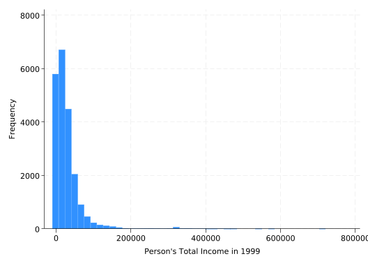
A histogram is a great tool for understanding the distribution of continuous variables, and you can create one with the hist command. Use the freq option to have the y-axis labeled in terms of frequency rather than density:
hist income, freq
(bin=43, start=-10000, width=16976.744)
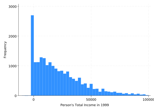
Unfortunately, the outliers drive the scale, making it hard to say much about the distribution of the bulk of the observations. Consider looking at a subset of the incomes:
hist income if income<100000, freq
(bin=43, start=-10000, width=2553.4884)
Exercise
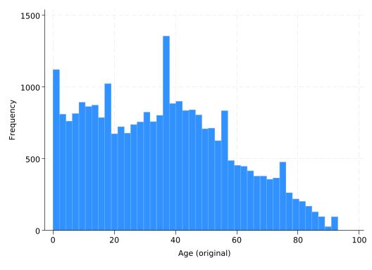
Examine the distribution of age using a histogram. How close is it to normally distributed? Do you see any anomalies? Since age is an integer, run another histogram with the discrete option, which gives you one bin for each value. Any concerns now?
Solution
hist age, freq
(bin=44, start=0, width=2.1136364)
No, definitely not a normal distribution. Note that the “baby boomers” in 2000 were between 34 and 54 years old, and they’re visible in the histogram.
hist age, freq discrete
(start=0, width=1)
The baby boomers are even easier to see with one bin for each value of age, but what really sticks out is the number of people with a value of 93 for age. That’s because age is top-coded: 93 actually means “93 or older.” This preserves anonymity since there are few people older than 93.
This would be a very important thing to know if your work with this data focused on the elderly! Looking closely at your data will give you a fighting chance to spot things like this, but the best way to learn about them is to read the data documentation.
3.13 Categorical Variables
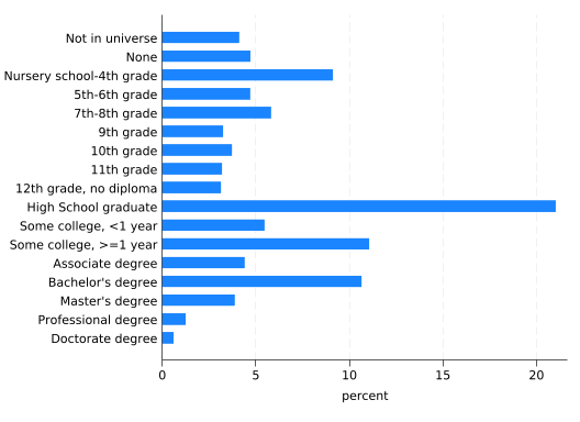
For a categorical variable like edu, tabulate (tab) is the place to start for understanding its distribution:
There are no missing values, or at least none coded as such.
The category “Not in universe” needs some investigation.
There are more people in lower education categories than you might expect (41.7% did not graduate from high school).
There may be more categories here than are useful, so consider combining them.
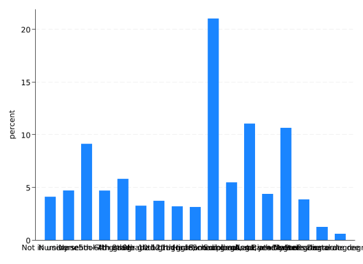
A bar graph is a great tool for understanding the distribution of categorical variables. Unlike a frequency table, a reader can absorb the information in a bar graph instantly. It may take some work to make them presentable; Bar Graphs in Stata discusses some of the tricks needed. You can see the problem if you try to create the default bar graph for edu:
graphbar, over(edu)
There’s not enough space on the x-axis for all the labels. But this problem has a very simple solution: switch to a horizontal bar graph.
graphhbar, over(edu)
This makes horizontal the format of choice for bar graphs.
The syntax for bar graphs may seem confusing: why the over() option rather than just graph hbar edu? The reason is that bar graphs are also used to examine relationships between variables. A variable list is used to specify the variable that defines the lengths of the bars (by default the mean of that variable), while the over() option specifies the variable that defines the bars themselves, as in:
graphhbar income, over(edu)
We hope the relative lengths of the last two bars do not surprise or disappoint any PhD students reading this.
Exercise
Examine the distribution of race.
Solution
tab race
            Race Recode 1 |      Freq.     Percent        Cum.
--------------------------+-----------------------------------
                    White |     20,636       75.29       75.29
                    Black |      3,202       11.68       86.97
          American Indian |        202        0.74       87.71
            Alaska Native |         15        0.05       87.76
Indigenous, tribe unknown |         64        0.23       87.99
                    Asian |        939        3.43       91.42
         Pacific Islander |         37        0.13       91.55
                    Other |      1,587        5.79       97.34
              Multiracial |        728        2.66      100.00
--------------------------+-----------------------------------
                    Total |     27,410      100.00
graphhbar, over(race)
Note that the US population has gotten a good bit less “white” since 2000.
3.14 Investigate Anomalies
We’ve identified several oddities in this data set as we’ve explored it. They could have significant effects on your analysis, so it’s important to figure out what they mean.
edu has a level called “Not in universe,” coded with 0. The Census Bureau probably isn’t actually collecting data on extra-dimensional beings, so what does this mean? Begin by examining the distribution of age for people who have “Not in universe” for edu:
sum age if edu==0
    Variable |        Obs        Mean    Std. dev.       Min        Max
-------------+---------------------------------------------------------
         age |      1,123    .9946572    .8076991          0          2
Everyone with “Not in universe” for education is under the age of three. Is the converse true?
tab edu if age<3
  Educational Attainment |      Freq.     Percent        Cum.
-------------------------+-----------------------------------
         Not in universe |      1,123      100.00      100.00
-------------------------+-----------------------------------
                   Total |      1,123      100.00
People with “Not in universe” are all under the age of three, and people under the age of three are always “Not in universe.” The Census Bureau uses “Not in universe” to mean the subject is not in the universe of people that the variable applies to; in this case it’s because if someone is under the age of three they don’t even ask about their education. “Legitimate skips” are similar: questions a respondent did not answer (skipped) because they did not apply.
This is why the different coding of hispan and asian in the ATUS is somewhat puzzling: hispan is treated as a categorical variable that applies to everyone, with one valid value being “Not Hispanic”; while asian is treated as a categorical variable that only applies to Asian people, with non-Asians being “Not in universe.” Either makes sense, but you’d expect them to be the same.
We also noted that the percentage of people with less than a high school education (41.7%) seemed high for the United States in 2000, but that includes children who simply aren’t old enough to have graduated from high school. If we limit the sample to adults the distribution is much more plausible:
This is a good example of how you should check your work as you go: see if your data matches what you know about the population of interest, and if not, be sure there’s a valid reason why.
We also noted negative values for income. First off, check how many there are:
countif income<0
29
Very few, which lowers the stakes in dealing with them. So who are the people with negative incomes?
sum age if income<0
    Variable |        Obs        Mean    Std. dev.       Min        Max
-------------+---------------------------------------------------------
         age |         29    49.89655    13.45454         24         77
  Person is |
     female |      Freq.     Percent        Cum.
------------+-----------------------------------
          0 |         16       55.17       55.17
          1 |         13       44.83      100.00
------------+-----------------------------------
      Total |         29      100.00
So they’re all adults, but there are no other obvious patterns. One plausible explanation is that these people had losses on investments and thus ended up with a negative value for total income. However, in order to lose money on investments you have to have investments. If that’s the explanation, these people may have substantial wealth even though they have negative incomes in this particular year. That’s problematic if you plan to use income as a proxy for broader socio-economic status. You might consider changing negative values of income to missing.
Exercise
Who are the people who marked “Other” for race? (Look at the distributions of other variables for the people who have “Other” for race.)
Solution
The first thing to do is remind yourself what the code for “Other” is. Remember we called the value labels for racerace_label, and then list it.
labellist race_label
race_label:
           1 White
           2 Black
           3 American Indian
           4 Alaska Native
           5 Indigenous, tribe unknown
           6 Asian
           7 Pacific Islander
           8 Other
           9 Multiracial
So we’re interested in the 8s.
Now there are lots of other variables you could look at, like age. age is continuous, so run summary statistics:
sum age if race==8
    Variable |        Obs        Mean    Std. dev.       Min        Max
-------------+---------------------------------------------------------
         age |      1,587    25.51292    17.04827          0         89
There’s nothing obvious going on there. How about hispanic? hispanic is categorical (more specifically an indicator) so this is a job for tab:
tab hispanic if race==8
  Person is |
   Hispanic |      Freq.     Percent        Cum.
------------+-----------------------------------
          0 |         58        3.65        3.65
          1 |      1,529       96.35      100.00
------------+-----------------------------------
      Total |      1,587      100.00
There we go: people who marked “Other” for race are almost all Hispanic.
To social scientists, race and ethnicity are different concepts, and someone who is Hispanic can also be white, Black, etc. But many people think of Hispanic as a race, so when they were asked to choose their race and didn’t see Hispanic there, they chose Other. The 2010 census changed the wording of the race question to try to clear this up.
On the other hand, race is a social construct anyway. So if people think of Hispanic as a race, for the purposes of a lot of social science research it makes sense to treat it as a race. For example, you could declare that a 10 for race will mean Hispanic, label it appropriately, and change race to 10 for everyone who said they were Hispanic.
You could call this variable something like race_eth in recognition that it includes both race and ethnicity. But the moment you remove the ability for someone to have both a race and an ethnicity, you’re not really treating race and ethnicity as separate things.
3.15 Recode Values that Mean Missing to Missing Values
Stata uses special codes to indicate missing values. For numeric values there’s the generic missing value, ., plus the extended missing values .a, .b, .c, through .z. (Recall that as far as greater than and less than are concerned, .<.a, .a<.b, etc. so if x<. excludes all missing values of x.) For strings, the empty string, "" (i.e. quotes with absolutely nothing inside, not even a space) means missing. These values receive special treatment. For example, statistical commands exclude missing values from their calculations.
Data sets often use different codes to indicate missing values. We saw that with income: “BBBBBBB” meant missing. This was automatically converted to a missing value when you converted income from a string variable to a numeric variable, but it won’t always be that simple. Recall that in the “harmonized” version of the ACS, 9999999 meant missing for income. It’s also common to use negative numbers to mean missing, especially -9. Stata will not recognize that a value like 9999999 means missing and will include it in statistical calculations, giving incorrect results.
The solution is to identify values that really mean missing, and then change them to missing values. For edu, the value 0, “Not in universe” means missing. Change it with:
replace edu = . if edu==0
(1,123 real changes made, 1,123 to missing)
What about negative values for income? Is that really a code for missing? Take a look with:
The variety of values suggest these are actual quantities, not codes.
Exercise
The codebook says that for marital_status 5 means “Never married (includes under 15 years).” In other words, the Census Bureau didn’t ask about the marital status of children under the age of fifteen just like they didn’t ask about the education of children under the age of three. But for marital status they coded it as if it were known that the children were never married. Undo this choice by changing marital_status to missing for children under fifteen.
Solution
replace marital_status = . if age < 15
(6,144 real changes made, 6,144 to missing)
3.16 Examine Missing Data
Once all missing values are coded in a way that Stata can recognize them, the misstable sum command will give you a very useful summary of the missing data in you data set.
misstable sum
                                                               Obs<.
                                                +------------------------------
               |                                | Unique
      Variable |     Obs=.     Obs>.     Obs<.  | values        Min         Max
  -------------+--------------------------------+------------------------------
  marital_st~s |     6,144              21,266  |      5          1           5
           edu |     1,123              26,287  |     16          1          16
        income |     6,144              21,266  |   >500     -10000      720000
  -----------------------------------------------------------------------------
Any variable that is not listed does not have any missing values. Thus you now know you can write conditions like if age>=65 without worrying about missing values of age being included–there aren’t any. You also see how many missing values you have for each variable, and thus how big an issue missing data is in your data set.
What misstable cannot tell you is why the data are missing. Sometimes you can answer this question by examining the relationships between missing values and other variables. For example, who are the people with missing values of income?
sum age if income==.
    Variable |        Obs        Mean    Std. dev.       Min        Max
-------------+---------------------------------------------------------
         age |      6,144    7.245117    4.315471          0         14
tab income if age<15, missing
   Person's |
      Total |
  Income in |
       1999 |      Freq.     Percent        Cum.
------------+-----------------------------------
          . |      6,144      100.00      100.00
------------+-----------------------------------
      Total |      6,144      100.00
The Census Bureau did not ask about the income of children under the age of 15 just like they did not ask about their marital status.
You should also consider relationships between missing values. In this data set, people with a missing value of income also have a missing value for marital_status because both variables were not collected for children under the age of 15. But in many data sets there are direct relationships between missing values. For example, if a subject could not be located in a wave of a survey then they may have missing values for all the variables for that survey wave.
Data is missing completely at random if the probability of it being missing is unrelated to either the observed data or the unobserved data. Thus the unobserved data has the same distribution as the observed data. Complete cases analysis (analysis of just the observed data) will have less power due to the missing data, but will be unbiased.
Data is missing at random if the probability of it being missing is related only to the observed data (the missingness is random conditional on the observed data.) Thus the unobserved data can be distributed differently from the observed data. Complete cases analysis will be biased, but methods such as weighting or multiple imputation may be able to correct that bias–though they generally depend on being able to make inferences about the unobserved data using the observed data. For example, pollsters know people with lower levels of education are less likely to respond to polls, but they can use the responses of those people with low levels of education who do respond to make inferences about those who don’t (typically by weighting).
Data is missing not at random if the probability of it being missing is related to the unobserved data. You cannot correct for bias due to missing not at random data; worse, you can’t even detect it using the observed data. For example, UW-Madison once did a survey on how much people use electronic calendars. The response rate was low and it seems likely that people who use calendars heavily would be more motivated to respond, meaning estimates of usage would be biased high. But there was no way to know for sure if this was true since the probability of answering the survey would thus depend on the values of usage that were not observed.
Consider edu, which is missing for children under the age of three. If we could observe the values of edu for these children, they would probably be mostly “None” with perhaps a few “Nursery school-4th grade” (presumably all “Nursery School”). This is very different from the observed distribution of edu. This is an example of “missing at random” since the probability of edu being missing depends on age and age is always observed, but it would be difficult to correct for the bias introduced because we have no actual data (just assumptions) about the distribution of edu for children under three.
Exercise
What is the likely distribution of income for people with a missing value for income? How would their mean income compare to the mean income of the people whose income was observed? How would the mean of income change if all its missing values became known? (In other words, how do the missing values of income bias estimates of the population mean of income?)
Solution
The people who have a missing value for income are all under 15 years of age, so their income is probably very low. The mean income of the people under 15 is almost certainly much lower than the mean income of the people who are 15 or older. So if we could observe everyone’s income, the mean value of income would be lower than we get now.
At this point the data set is reasonably clean, and what you do with it next will depend on how you plan to use it. For example, if you wanted to use education as a predictor in a regression model it would probably be wise to combine some of the categories, but if you were doing a descriptive study you might leave it as is. Wrap up this do file by saving the cleaned-up data set (never saving it over the original file) and closing the log:
save 2000_acs_clean, replacelogclose
file 2000_acs_clean.dta saved
      name:  <unnamed>
       log:  /home/d/dimond/kb/dws/first_steps_examples.log
  log type:  text
 closed on:  24 Nov 2025, 17:16:58
-------------------------------------------------------------------------------
// tempsave acs, replacereshapewide age edu race female hispanic income marital_status, i(household) j(person)save acs_wide, replace
file acs.dta saved
(j = 1 2 3 4 5 6 7 8 9 10 11 12 13 14 15 16)

Data                               Long   ->   Wide
-----------------------------------------------------------------------------
Number of observations           27,410   ->   10,565
Number of variables                   9   ->   113
j variable (16 values)           person   ->   (dropped)
xij variables:
                                    age   ->   age1 age2 ... age16
                                    edu   ->   edu1 edu2 ... edu16
                                   race   ->   race1 race2 ... race16
                                 female   ->   female1 female2 ... female16
                               hispanic   ->   hispanic1 hispanic2 ... hispanic
> 16
                                 income   ->   income1 income2 ... income16
                         marital_status   ->   marital_status1 marital_status2
> ... marital_status16
-----------------------------------------------------------------------------
file acs_wide.dta saved
Review
As a review, here are the first steps you should take with your data. Many of them are very quick; and the ones that take more time are especially valuable. Do not skip these steps!
Read the Documentation
Identify the Variables
Look at the Data
Find the Identifiers and Figure Out the Data Structure
Get Rid of Data You Won’t Use
Change Variable Names
Convert String Variables that Contain Numbers to Numeric Variables