10 Reading Text Data
A typical project begins by reading data from somewhere into a data frame. A typical data source might be a text file, but it is also possible to import data from binary data files such as those used by Stata, SAS, and SPSS.
Text files come in many forms. It is always a good idea to look at any documentation you have first. Then it can be informative to look at the text file itself, preferably in a dedicated text editor (on SSCC computers, use Notepad++).
10.1 Text Data Concepts
You are looking for a few things when you examine the file.
Data, metadata, extra text
The file includes data values. Does it also include variable names or other information that helps define the data? Is there a header or a footer with explanatory text about the file contents?
Observation delimiter
What separates one observation from the next? Commonly, each observation has a separate line in the text file, but it is possible to have multiple observations per line, or multiple lines per observation.
Data value delimiter
Within an observation, what separates one data value from the next? Very commonly the data value delimiter will be a space or a comma. Tabs used to be common, and are hard to distinguish visually from spaces.
Especially in older data sets, it used to be common for data values to appear in specified columns - e.g. state in columns 3-4 and county in columns 5-7 - with no character delimiting data values.
Character value quote
Where data value delimiters are used, how are the same characters included in character data values? For instance, if the data values are separated by spaces, how do you include a space within a data value? The typical answer is, character data values are enclosed in quotes, either double (") or single (’) quotes.
Missing value string
How are missing values indicated? This might be by having two data value delimiters with no data value between them. Or there might be a special string that denotes missing data, such as NA, -99, or BBBBBBB. There may be more than one missing value indicator as well, such as -98 and -99.
10.2 Reading Data Files
10.2.1 CSV Examples
10.2.1.1 The Simple Case
Consider this file:
fn <- "https://www.ssc.wisc.edu/~hemken/Rworkshops/read/class.csv"The first few lines look like this:
Name,Sex,Age,Height,Weight
Alfred,M,14,69,112.5
Alice,F,13,56.5,84
Barbara,F,13,65.3,98
Carol,F,14,62.8,102.5
Henry,M,14,63.5,102.5
In this file,
- The first line has variable names, and the rest is data.
- There is one observation per line.
- Data values are separated by commas.
- There appear to be no character quotes.
- There appear to be no missing values.
Data like this is very easy to read into R with the read.csv() function:
class <- read.csv(fn)
head(class)
Name Sex Age Height Weight
1 Alfred M 14 69.0 112.5
2 Alice F 13 56.5 84.0
3 Barbara F 13 65.3 98.0
4 Carol F 14 62.8 102.5
5 Henry M 14 63.5 102.5
6 James M 12 57.3 83.0str(class)'data.frame': 19 obs. of 5 variables:
$ Name : chr "Alfred" "Alice" "Barbara" "Carol" ...
$ Sex : chr "M" "F" "F" "F" ...
$ Age : int 14 13 13 14 14 12 12 15 13 12 ...
$ Height: num 69 56.5 65.3 62.8 63.5 57.3 59.8 62.5 62.5 59 ...
$ Weight: num 112 84 98 102 102 ...10.2.1.2 Characters to Factors
Prior to R-4.0, Name and Sex in the previous example would have been turned into factors automatically. This is no longer the default, but remains an option.
class <- read.csv(fn, as.is=FALSE) # all character vars to factors
#head(class)
str(class)
'data.frame': 19 obs. of 5 variables:
$ Name : Factor w/ 19 levels "Alfred","Alice",..: 1 2 3 4 5 6 7 8 9 10 ...
$ Sex : Factor w/ 2 levels "F","M": 2 1 1 1 2 2 1 1 2 2 ...
$ Age : int 14 13 13 14 14 12 12 15 13 12 ...
$ Height: num 69 56.5 65.3 62.8 63.5 57.3 59.8 62.5 62.5 59 ...
$ Weight: num 112 84 98 102 102 ...To convert specific columns to factors, do the conversion as a separate step later,
or use a named vector of column classes in a colClasses argument.
The vector values are classes to assign, the names are variable names:
cc <- c(Sex="factor") # a named vector of column classes
class <- read.csv(fn, colClasses = cc)
#head(class)
str(class)
'data.frame': 19 obs. of 5 variables:
$ Name : chr "Alfred" "Alice" "Barbara" "Carol" ...
$ Sex : Factor w/ 2 levels "F","M": 2 1 1 1 2 2 1 1 2 2 ...
$ Age : int 14 13 13 14 14 12 12 15 13 12 ...
$ Height: num 69 56.5 65.3 62.8 63.5 57.3 59.8 62.5 62.5 59 ...
$ Weight: num 112 84 98 102 102 ...10.2.1.3 No Header
Now consider this file:
fnnh <- "https://www.ssc.wisc.edu/~hemken/Rworkshops/read/classnh.csv"The first few lines look like this:
Alfred,M,14,69,112.5
Alice,F,13,56.5,84
Barbara,F,13,65.3,98
Carol,F,14,62.8,102.5
Henry,M,14,63.5,102.5
James,M,12,57.3,83
The default use of read.csv() takes the first line to be variable
names, resulting in some nonsense names:
classnh <- read.csv(fnnh)
#head(classnh)
str(classnh)
'data.frame': 18 obs. of 5 variables:
$ Alfred: chr "Alice" "Barbara" "Carol" "Henry" ...
$ M : chr "F" "F" "F" "M" ...
$ X14 : int 13 13 14 14 12 12 15 13 12 11 ...
$ X69 : num 56.5 65.3 62.8 63.5 57.3 59.8 62.5 62.5 59 51.3 ...
$ X112.5: num 84 98 102 102 83 ...We now need a header=FALSE argument. We can optionally add a
col.names argument, or add names()<- in a separate step, later.
classnh <- read.csv(fnnh, header=FALSE)
str(classnh) # default names
'data.frame': 19 obs. of 5 variables:
$ V1: chr "Alfred" "Alice" "Barbara" "Carol" ...
$ V2: chr "M" "F" "F" "F" ...
$ V3: int 14 13 13 14 14 12 12 15 13 12 ...
$ V4: num 69 56.5 65.3 62.8 63.5 57.3 59.8 62.5 62.5 59 ...
$ V5: num 112 84 98 102 102 ...classnh <- read.csv(fnnh, header=FALSE, col.names = c("name", "sex", "age",
"ht", "wt"))
str(classnh)'data.frame': 19 obs. of 5 variables:
$ name: chr "Alfred" "Alice" "Barbara" "Carol" ...
$ sex : chr "M" "F" "F" "F" ...
$ age : int 14 13 13 14 14 12 12 15 13 12 ...
$ ht : num 69 56.5 65.3 62.8 63.5 57.3 59.8 62.5 62.5 59 ...
$ wt : num 112 84 98 102 102 ...10.2.1.4 Quoted Character Values
Quoting character values is seldom a problem … but sometimes it is. So consider this file:
fnq <- "https://www.ssc.wisc.edu/~hemken/Rworkshops/read/classq.csv"The first few lines look like this:
"Name","Sex","Age","Height","Weight"
"B, Alfred","M",14,69,112.5
"Y, Alice","F",13,56.5,84
"M, Barbara","F",13,65.3,98
"P, Carol","F",14,62.8,102.5
"A, Henry","M",14,63.5,102.5
This is what we’d like to see. There are commas within the data values
for Name, but these are all in quotes. The default use of read.csv()
assumes that double quotes or single
quotes delimit character values. If some other character is used, we have
the quote argument we can use. If nothing is used, we could be in trouble!
(We might need a new strategy.)
classq <- read.csv(fnq)
str(classq)
'data.frame': 19 obs. of 5 variables:
$ Name : chr "B, Alfred" "Y, Alice" "M, Barbara" "P, Carol" ...
$ Sex : chr "M" "F" "F" "F" ...
$ Age : int 14 13 13 14 14 12 12 15 13 12 ...
$ Height: num 69 56.5 65.3 62.8 63.5 57.3 59.8 62.5 62.5 59 ...
$ Weight: num 112 84 98 102 102 ...10.2.1.5 Missing Values
Next, consider this file:
fnm <- "https://www.ssc.wisc.edu/~hemken/Rworkshops/read/classm.csv"The first few lines look like this:
Name,Sex,Age,Height,Weight
Alfred,M,14,,112.5
Alice,F,13,56.5,84
Barbara,F,13,65.3,98
Carol,F,14,62.8,102.5
Henry,M,14,63.5,102.5
Here we have a missing value for Height in the first observation (and more later in the data set).
classm <- read.csv(fnm)
head(classm)
Name Sex Age Height Weight
1 Alfred M 14 NA 112.5
2 Alice F 13 56.5 84.0
3 Barbara F 13 65.3 98.0
4 Carol F 14 62.8 102.5
5 Henry M 14 63.5 102.5
6 James M 12 57.3 83.0Depending on the software used to produce the text file, a missing value
might be denoted by two data delimiters with no text in between, as in
this example. In text files produced by R iteself, missing values
are usually denoted by NA. So by default these are turned into missing
values as well. Other software might use another symbol (periods are common,
and dashes sometimes are used), for which we have the na.strings argument.
10.2.2 Space Delimited
For space delimited data, we use a related function, read.table(). Here
a few of the assumptions (defaults) are different. Now spaces are assumed
to delimit data values where before they were assumed to be part of data
values, and vice versa for commas. Files are assumed to have no headers.
The other major arguments work as before.
fnsp <- "https://www.ssc.wisc.edu/~hemken/Rworkshops/read/class.txt"The first few lines look like this:
Name Sex Age Height Weight
Alfred M 14 69 112.5
Alice F 13 56.5 84
Barbara F 13 65.3 98
Carol F 14 62.8 102.5
Henry M 14 63.5 102.5
Here we have a header with variable names, which we need to indicate.
classm <- read.table(fnsp, header=TRUE)
str(classm)
'data.frame': 19 obs. of 5 variables:
$ Name : chr "Alfred" "Alice" "Barbara" "Carol" ...
$ Sex : chr "M" "F" "F" "F" ...
$ Age : int 14 13 13 14 14 12 12 15 13 12 ...
$ Height: num 69 56.5 65.3 62.8 63.5 57.3 59.8 62.5 62.5 59 ...
$ Weight: num 112 84 98 102 102 ...10.2.3 Fixed-Width Text
Data in fixed columns is easy to recognize when the data values run together. Even if they do not, this can be a solution when spaces or commas are valid data values and there are no character value quotes. Missing values are typically spaces, as well.
fnfw <- "https://www.ssc.wisc.edu/~hemken/Rworkshops/read/classfw.txt"The first few lines look like this:
Alfred M1469  112.5
Alice  F1356.584
BarbaraF1365.398
Carol  F1462.8102.5
Henry  M1463.5102.5
James  M1257.383
Here we need to know how many columns each variable occupies (including spaces). Data documentation is a huge help here.
Notice that the width includes the decimal character.
widths <- c(7,1,2,4,5)   # how many columns wide each of the variables is

classfw <- read.fwf(fnfw, widths)
head(classfw)
V1 V2 V3 V4 V5
1 Alfred M 14 69.0 112.5
2 Alice F 13 56.5 84.0
3 Barbara F 13 65.3 98.0
4 Carol F 14 62.8 102.5
5 Henry M 14 63.5 102.5
6 James M 12 57.3 83.010.3 Writing Data Files
After you have read in and manipulated your data in R, you should save your data. As you might have guessed, the opposite of read.csv() is write.csv().
The write.csv() function has the default option of row.names = T, which will create a column with our row names. Since we did not name the rows in classfw, they contain the default vector of 1:nrow(classfw) by default. If we do not want this, we can specify row.names = F.
write.csv(classfw, "classfw.csv", row.names = F)To customize the separators and file format, see help(write.table).
You may also choose to save your data in the .RData format. R is able to read this file type faster than CSVs, but the disadvantage is that you cannot easily preview the file in application such as Excel or a text editor. With smaller datasets, you may not notice a difference in loading time. However, if you work with larger datasets, you may be able to save a lot of time by using .RData files.
save(classfw, file = "classfw.RData")To load the file back into R,
load("classfw.RData")Note that you do not have to assign the result of load() to another variable as you do with read.csv() and other functions.
10.4 Paths and Working Directories
Data files have a name and are located in a folder. (A folders is the same a directory. You will see both of these names in common use.) The folder containing the file may be nested within another folder and that folder maybe in yet another folder and so on. The specification of the list of folders to travel and the file name is called a path. A path that starts at the root folder of the computer is called an absolute path. A relative path starts at a given folder and provides the folders and file starting from that folder. Using relative paths will make a number of things easier when writing programs and is considered a good programming practice.
A path is made up of folder names. If the path is to a file, then the path will ends with a file name. The folders and files of a path are separated by a directory separator (e.g., / or \). Different operating systems use different directory separators. In R, the function file.path() is used to fill in the directory separator. It knows which separator to use for the operating system it is running on.
There are a few special directory names. A single period, ., indicates the current working directory. Two periods, .., indicates moving up a directory. The following image shows how .. would be used to get a data file in the folder structure used in the project organization section.
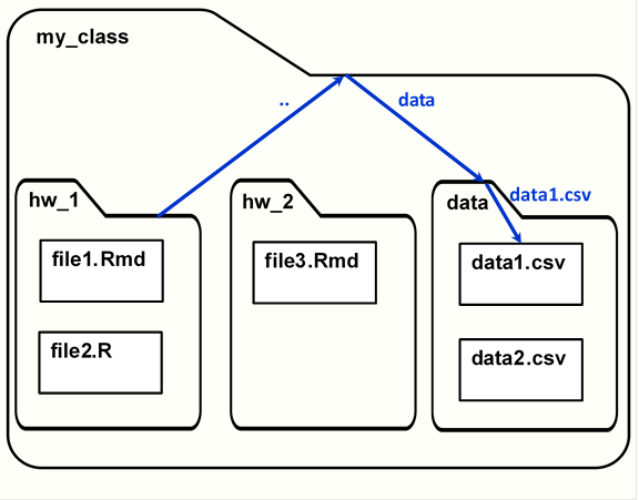
Relative file paths.
When R starts a session, it has a location to look for other files. This path is called the current working directory, and this is often shortened to the working directory. Relative paths in a program are specified as starting at the current working directory. To print your current working directory, use the getwd() function. To change your working directory, supply setwd() with a relative path in quotes (or an absolute path, but relative paths are preferred).
getwd()[1] "U:/school/my_class"setwd("hw_1")In the image above, if your working directory is the folder hw_1, you can reach the data1.csv file with the path “../data/data1.csv”. This path could be given to read.csv() (or another data-reading function) to read in the data, or to write.csv() to write over the file.
You can also have file.path() create file paths for you:
data_path <- file.path("..", "data", "data1.csv")
data_path
[1] "../data/data1.csv"And then use the objects created by file.path() to make reading and writing files simpler:
read.csv(data_path)

# create a partial path so we can customize the file name
data_folder <- file.path("..", "data")

# path is "../data/data1.csv"
read.csv(file.path(data_folder, "data1.csv"))

# path is "../data/data2.csv"
write.csv(dat, file.path(data_folder, "data2.csv"))
10.5 Reading Exercises
Set your working directory to your Desktop.
With
dir.create(), create a folder called “Project”. Then, inside of “Project”, create three folders: “Data_raw”, “Data_formatted”, and “Scripts”.Download a dataset from the Census (try not to pick a CSV file) and drag-and-drop it into the Data_raw folder.
Set your working directory to the Scripts folder.
Create a new R script and save it in Scripts.
Without changing your working directory from Scripts, read in your downloaded file from Data_raw and then save it as a CSV file to Data_formatted. Save these commands in your R script.
This is the beginning of a well-organized project!