9 Categorical Data

We generally think of data as a collection of “measurements,” in a loose sense of the word “measurement”. In this loose sense, there are two basic types of “measurement”, measurements on continuous scales, and measurements on categorical scales. (In ordinary speech the word “measurement” often implies a continuous scale.)

Continuous measurements can be represented by a point on a number line, are well-ordered, and in principle can take on one value of an infinite set of choices. Think of a variable like age, which varies continuously from 0 to higher numbers, and where there is a unique order to the ages represented by 1, 5.5, and 55. In principle we can measure age with arbitrary precision - 5.5, or 5.5001 or 5.5000001. The scale here might be measured in days or years, but in any case it is continuous.

Categorical measurements can be represented by arbitrary labels (maybe numerals, maybe character strings), have no conceptual order, and take one value from a finite set of choices. Think of a variable like state of residence, which takes one of about 50 values (Washington, D.C.? Territories?), which have no inherent order.

(Interval and ordinal measurements may be thought of, and are often treated, as continuous measurements with limited precision.)

The distinction between continuous and categorical variables is fundamental to how we use them the analysis. In a regression for example, continuous variables give us slopes and curvature terms, where categorical variables give us intercepts.

In R, it is convenient to manage categorical data as factors. In software like Stata, SAS, and SPSS, we specify which variables are categorical when we call an analytical procedure like regression - no special distinction is made when we are managing or storing our data. In R, we specify which variables are factors when we create and store them - in an analytical procedure we need make no additional specification to distinguish levels of measurement.

In R, a factor refers to a class of data stored in numeric form, usually with some sort of values labels. The numbers (integers) merely represent distinct categories, with no meaningful order to the categories.

For example, we might have a data set where ‘1’ means Green Bay, ‘2’ means Madison, and ‘3’ means Milwaukee.

As with Date class data, we will seldom need to manipulate the underlying integers, we will mainly work with the “human-readable” value labels.

The basic constructor function for data with class ‘factor’ is factor(). For example, we can begin with a character vector of city names, and use factor() to construct a factor from this.

city <- c("Madison", "Milwaukee", "Green Bay")
city
[1] "Madison"   "Milwaukee" "Green Bay"
x <- factor(city)
x
[1] Madison   Milwaukee Green Bay
Levels: Green Bay Madison Milwaukee

Notice that factors print differently than character data - no quotes.

9.1 Factors in Generic Functions

In addition to printing slightly differently than character data, in generic functions that take numeric inputs, factors are treated differently as well. Three functions that give different output with factors (versus a numeric vector) are summary(), plot(), and lm().

We can look at the example data set chickwts, which includes both a numeric variable and a factor variable. We learn from help(chickwts) that this data set was created from an experiment testing the effect of different feeds on chicken weights.

Using the summary function, the factor feed produces a frequency table, rather than the six number summary produced by weight.

str(chickwts)   # "weight" is numeric, "feed" is categorical
'data.frame':   71 obs. of  2 variables:
 $ weight: num  179 160 136 227 217 168 108 124 143 140 ...
 $ feed  : Factor w/ 6 levels "casein","horsebean",..: 2 2 2 2 2 2 2 2 2 2 ...
head(chickwts)
  weight      feed
1    179 horsebean
2    160 horsebean
3    136 horsebean
4    227 horsebean
5    217 horsebean
6    168 horsebean

summary(chickwts)
     weight             feed   
 Min.   :108.0   casein   :12  
 1st Qu.:204.5   horsebean:10  
 Median :258.0   linseed  :12  
 Mean   :261.3   meatmeal :11  
 3rd Qu.:323.5   soybean  :14  
 Max.   :423.0   sunflower:12

In plots, a factor produces a categorical x-axis, and a boxplot rather than a scatter plot.

plot(weight ~ feed, data=chickwts)

In modeling, a factor is used as a categorical variables, generating a set of dummy variables and a set of parameters, rather than a single parameter.

summary(lm(weight ~ feed, data=chickwts))


Call:
lm(formula = weight ~ feed, data = chickwts)

Residuals:
     Min       1Q   Median       3Q      Max 
-123.909  -34.413    1.571   38.170  103.091 

Coefficients:
              Estimate Std. Error t value Pr(>|t|)    
(Intercept)    323.583     15.834  20.436  < 2e-16 ***
feedhorsebean -163.383     23.485  -6.957 2.07e-09 ***
feedlinseed   -104.833     22.393  -4.682 1.49e-05 ***
feedmeatmeal   -46.674     22.896  -2.039 0.045567 *  
feedsoybean    -77.155     21.578  -3.576 0.000665 ***
feedsunflower    5.333     22.393   0.238 0.812495    
---
Signif. codes:  0 '***' 0.001 '**' 0.01 '*' 0.05 '.' 0.1 ' ' 1

Residual standard error: 54.85 on 65 degrees of freedom
Multiple R-squared:  0.5417,    Adjusted R-squared:  0.5064 
F-statistic: 15.36 on 5 and 65 DF,  p-value: 5.936e-10

Here, all the categorical parameters are named with the prefix “feed”.

9.2 Logical Comparisons and Math Operators

Logical comparisons are made with the value labels (which are character strings), not the underlying integer codes. Only some logical operators are allowed with factors, namely those based on equality.

rs <- sample(chickwts$feed, 7)
rs
[1] sunflower horsebean soybean   sunflower sunflower soybean   horsebean
Levels: casein horsebean linseed meatmeal soybean sunflower
rs == "casein"
[1] FALSE FALSE FALSE FALSE FALSE FALSE FALSE
rs == 1  # no error message, but WRONG!
[1] FALSE FALSE FALSE FALSE FALSE FALSE FALSE
rs > "casein" # error
Warning in Ops.factor(rs, "casein"): '>' not meaningful for factors
[1] NA NA NA NA NA NA NA

Notice that if we try to check for a numeric value, the numeral is treated as if it were a label and not the underlying data! It would be nice if this at least gave us a warning!

In a similar manner, we will not be doing any math at all with categorical data.

rs + 1
Warning in Ops.factor(rs, 1): '+' not meaningful for factors
[1] NA NA NA NA NA NA NA
mean(rs)
Warning in mean.default(rs): argument is not numeric or logical: returning NA
[1] NA

9.3 Levels and Labels

The factor() function has two key arguments: levels and labels.

There is a crucial difference between these two arguments. The levels parameter sets the order. The labels parameter assigns value labels to the “given” order. If no levels are specified, the order is sorted alphabetically (which is seldom what we want).

As an example, we can make a new copy of the feed variable with the levels reordered (“re-leveled”, this is also called “re-factoring”):

chick <- chickwts          # first, create a working copy
chick$feed2 <- factor(chick$feed, levels=
                           c("horsebean", "linseed", "soybean",
                             "meatmeal", "casein", "sunflower"))
plot(weight ~ feed2, data=chick, main="Reordered levels")

If we attempt to use the labels argument, we merely relabel the data (which in this case is WRONG!):

chick$feed3 <- factor(chick$feed, labels=
                           c("horsebean", "linseed", "soybean",
                             "meatmeal", "casein", "sunflower"))

opar <- par(mfcol=c(2,1))
plot(weight ~ feed, data=chick, main="Original")
plot(weight ~ feed3, data=chick, main="Bad labels")

par(opar)

Think of levels as an “input” function, specifying what numbers to use to encode categories. Then labels is an “output” function, specifying how the underlying data should be displayed.

One other useful function here, to slightly reorder the levels so that we have a new category in the first position, is the relevel() function.

chick$feed4 <- relevel(chick$feed, "sunflower")
plot(weight ~ feed4, data=chick, main="New first level")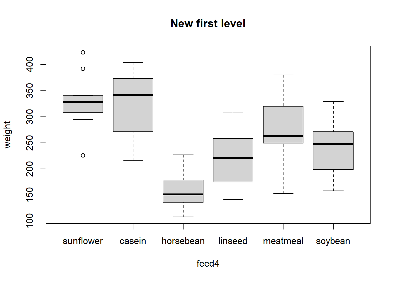

In practice, there are many different ways we might want to reorder (recode) the levels of a factor. The package forcats from the tidyverse collection of packages has quite a few useful functions for this.

9.4 Collapsing and Dropping Categories

To combine several categories of an existing factor into one category, we relabel them.

While we use the labels to combine categories, notice that the underlying integers are also recoded.

chick$feed5 <- factor(chick$feed, labels=
                           c("A", "A", "A",
                             "B", "B", "B"))
plot(weight ~ feed5, data=chick)

str(chick$feed5)

 Factor w/ 2 levels "A","B": 1 1 1 1 1 1 1 1 1 1 ...

If you have a lot of categories, but only a few to combine, the forcats function fct_recode() is very useful.

To drop categories, just do not mention them among the input levels. The data is encoded <NA>, the missing value.

chick$feed6 <- factor(chick$feed, levels=
                           c("horsebean", "casein"))
plot(weight ~ feed6, data=chick)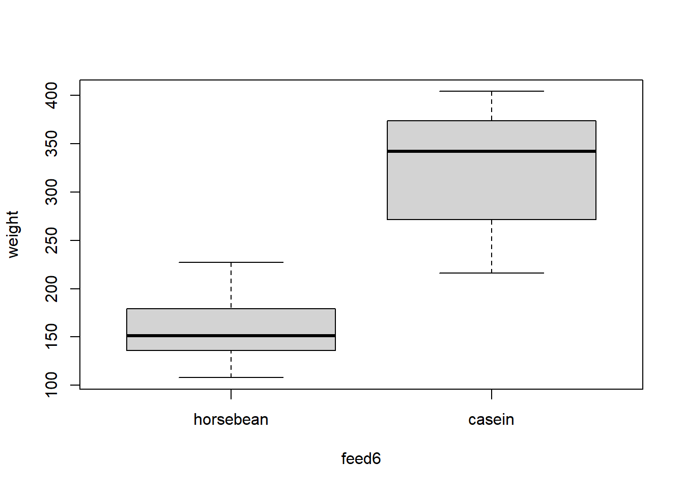

table(chick$feed, chick$feed6, useNA="ifany")

           
            horsebean casein <NA>
  casein            0     12    0
  horsebean        10      0    0
  linseed           0      0   12
  meatmeal          0      0   11
  soybean           0      0   14
  sunflower         0      0   12

9.5 A confusing function name

Just to make things confusing, the levels() function returns and sets the level labels

chick$feed2 <- chick$feed
levels(chick$feed)  # what we have

[1] "casein"    "horsebean" "linseed"   "meatmeal"  "soybean"   "sunflower"

# sets WRONG! labels again
levels(chick$feed2) <-c("horsebean", "linseed", "soybean",
                          "meatmeal", "casein", "sunflower")
plot(weight ~ feed2, data=chick, main="Bad labels again")

9.6 Categorical Vector Exercises

Convert Numeric Codes to Factors

In the mtcars data, all the variables are numeric. Convert vs to a factor, where 0 has the label “V-shaped” and 1 has the label “Straight”. How are the levels encoded, numerically?

Do the same for am, giving 0 the label “automatic” and 1 the label “manual”.
Extract and Convert Row Names

Again in mtcars, take the row.names and extract the make of each car type (the first word in the row name). Convert this into a factor.

Produce a frequency count of each car maker.

Plot car weight (wt) over car make.

Re-level so that Maserati is the first category, then replot.
Superfluous Levels

If is quite possible to have a factor defined with extra levels, levels for which you have labels but no actual data. Here is an example:
```
x <- sample(c("A", "B"), 20, replace=TRUE)
xf <- factor(x, levels=c("A", "B", "C"))
```
Produce a table of frequency counts for xf.

Produce a bar chart of counts, plot(xf).

For most analyses, we would rather drop the extra category. The simplest approach is to refactor, without specifying levels or labels.

Try
```
xf2 <- factor(xf)
```
Then retabulate and replot.