11 Latent Profile Analysis Basics
Latent profile analysis (LPA) can be thought of as a special form of latent class analysis where all the measurement variables are continuous.
In MPlus, the most basic LPA can be specified simply by declaring a CLASSES variable name with the number of categories that variable will have in parentheses. This is included in the VARIABLE section of the input file.
Then you must also specify that the analysis type is a MIXTURE.
If you would like to try the examples, the data is here.
11.1 Equal Variances
DATA:
    file = LPA_twoclass.dat;
VARIABLE:
    names = V1-V5;
    classes=c(2);
ANALYSIS:
    type=mixture;
The default model here is a two class model in which all the input variables are assumed to be normally distributed. This model also assumes that the variances of each measure are equal across the classes.
It is sometimes helpful to go ahead and write a MODEL section that makes the default assumptions explicit. This can be a helpful reminder when you come back to a project after a break, and will also make it easier to relax or impose other assumptions, if you decide to refine the model.
An explicit version of the previous model could be written in a number of different ways. Here is one way that strikes a balance between succinct notation and explicit defaults.
DATA:
    file = twoclass.dat;
VARIABLE:
    names = V1-V5;
    classes=c(2);
ANALYSIS:
    type=mixture;
MODEL:
    %OVERALL%
        V1-V5;   ! item variances, both classes;
    %C#1%
        [V1-V5]; ! item means, class one;
    %C#2%
        [V1-V5]; ! item means, class two;
Uncorrelated variables
This model will produce a warning:
*** WARNING in MODEL command
  All variables are uncorrelated with all other variables within class.
  Check that this is what is intended.
For a classic LPA, you do intent the variables to be uncorrelated within each class - in LPA this “warning” is good, telling you the model is correctly specified.
How many measures do you need?
The answer to this question depends on the data. It would be possible for a single measure to show complete separation between the two classes, so the software only requires one measurement variable. However, if a single measure gave you such clear separation, you wouldn’t really need LPA to distinguish which observations belong to which class. More measures related to the latent classes are usually a good thing, improving class entropy.
MPlus reports entropy in the MODEL FIT INFORMATION section of the output.
CLASSIFICATION QUALITY
     Entropy                         0.940
Like an R-squared in linear models, entropy is best thought of as a measure of model quality - a higher number is better, but it is not useful in hypothesis testing. For researchers who will be doing further analysis based on the estimated classes, low entropy increases the uncertainty inherent in any further estimation, and values above 0.8 or 0.9 are usually desired.
11.2 Unequal Variances
To relax the assumption of equal measure variances, you must specify separate sub-models for each class. This now requires sections for %C#1% and %C#2%, which were optional above. (This model could also include an %OVERALL% section, but that is still optional here.)
DATA:
    file = twoclass.dat;
VARIABLE:
    names = V1-V5;
    classes=c(2);
ANALYSIS:
    type=mixture;
MODEL:
    %C#1%
        V1-V5;
    %C#2%
        V1-V5;
11.3 Other Equality Constraints
Other equality constraints can be imposed in the usual way, by adding labels to specific parameters, and using the same label for parameters that are assumed to be equal.
11.4 Additional Parameters
You can calculate additional parameters that are derived from your model by adding a MODEL CONSTRAINT section to your code, and specifying how the additional parameter is calculated from the basic model parameters through the use of labels.
For example, if you wanted to calculate the difference between the mean of V1 in class 1 and the mean of V1 in class 2, your code could be
VARIABLE:
    names = V1-V5;
    classes=c(2);
ANALYSIS:
    type=mixture;
MODEL:
    %C#1%
        [V1] (a);
    %C#2%
        [V1] (b);
MODEL CONSTRAINT:
    NEW diff;
    diff = b - a;
The mean [V1] is given a different label in class 2 than in class 1, so that we can use the labels in the MODEL CONSTRAINT section. Notice that the means [V2-V5] are not mentioned in the MODEL section, nor are the variances V1-V5, so they will be set by their default assumptions.
11.5 Stabilizing Class Representation
Because estimating the class model makes use of an initial random process, the order in which classes are reported in the output can change from run to run. This just makes interpreting your results more work. To avoid this instability in the class order, many researchers will assign starting values to each class. It helps to have an initial LPA to figure out what starting values will be useful.
In this example, I’ve looked at previous results to see that one class has negative means on all the measures, while the other class has positive means on all the measures. This observation allows me to use a very succinct specification to ensure that the “positive” class is reported first.
Notice in this model that I am reverting to equal measure variances, and only specifying starting values for the means. This does not change my results, it only ensures the order in which the classes are reported.
DATA:
    file = twoclass.dat;
VARIABLE:
    names = V1-V5;
    classes=c(2);
ANALYSIS:
    type=mixture;
MODEL:
    %C#1%
        [V1-V5*1];
    %C#2%
        [V1-V5*-1];
12 Comparing Classification Models
An exploratory LPA will often begin by trying to verify the number of latent classes. There are several measures that researchers may consider when asking what number of classes optimizes the observed data. Perhaps the most widespread approach is to look at the likelihood measures associated with models of different numbers of classes, especially AIC and BIC.
For example, from the above model
| Model | AIC | BIC | Entropy |
|---|---|---|---|
| One class | 28038.601 | 28094.610 | (undefined) |
| Two classes | 24305.662 | 24395.276 | 0.940 |
| Three classes | 24308.864 | 24432.084 | 0.638 |
Results that are not crystal clear are more common than most researchers would like. AIC and BIC may suggest different models are optimal. Or there may not be much difference between the scores for two models, as is the case here. While the two class model has a very slight edge with AIC and BIC, we also see that the entropy is much higher with the two class model - the classes are more clearly separated. The theory underlying the models is especially important to consider as well.
MPlus offers two other diagnostic tests as well: the Vuong-Lo-Mendell-Rubin likelihood ratio test, and a bootstrapped likelihood ratio test. Both of these test a null hypothesis of \(k-1\) versus an alternative of \(k\) classes (where \(k\) is the number of classes specified in your code). See the MPlus web note 14 (Asparouhov & Muthen, 2012) which describes the methods as well as additional options.
You request these with the TECH11 and TECH14 options in the OUTPUT section of your code.
OUTPUT:
    tech11;
    tech14;
From the above models we get
| Model | VLMR p-value | BLRT p-value |
|---|---|---|
| Two classes (versus 1) | 0.0000 | 0.0000 |
| Three classes (versus 2) | 0.4829 | 0.6667 |
We see that the null hypothesis of \(k-1=1\) versus the alternative of \(k=2\) is rejected by both tests. Additionally, the null hypothesis of \(k-1=2\) versus the alternative of \(k=3\) is not rejected by either test. This, along with our theory, reinforces the judgement from AIC and BIC that there are two latent classes.
13 Measure Profile Plots
13.1 Basic MPlus plots
MPlus includes the capability of creating basic plots, and among these is a plot showing the estimated mean values of each measure in each class. For the above model we could create a graph like this
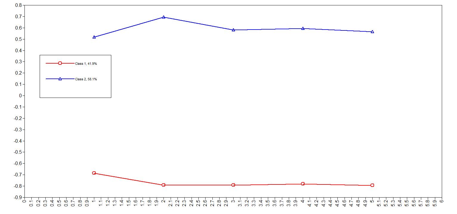
While most people would not consider this publication quality, it can be very useful for understanding your data.
To create this sort of plot, you need to
- include a PLOT section in your code
- use the MPlus graphical user interface to generate the plot
- optionally, save the plot
In this case, the PLOT section requests either plots2 or plots3. You also specify the X value used to represent each measure, creating a series of points that will be connected with a line.
PLOT:
    type=plot2;
    series = V1 (1) V2 (2) V3 (3) V4 (4) V5 (5);
Once the model has been estimated, in the MPlus GUI use the menus Plot > View plots
In the dialog box, select Estimated means, medians, modes, and percentiles
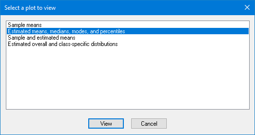
And in a second dialog box, use the default options.

13.2 Export Graph Data
If you would like to redraw this graph in other software to produce a publication-worthy graph, you can save the graph data by going back to the Plot menu
Plot > Save plot data
This produces a simple text file that you can import into any other statistical software.