With the sequence of uniform random numbers, we next transform them to a distribution of interest. Let (F) represent a distribution function of interest. Then, use the inverse transform
[
X_i=F^{-1}left( U_i right) .
]
The result is that the sequence {(X_{i})} is approximately i.i.d. with distribution function (F).
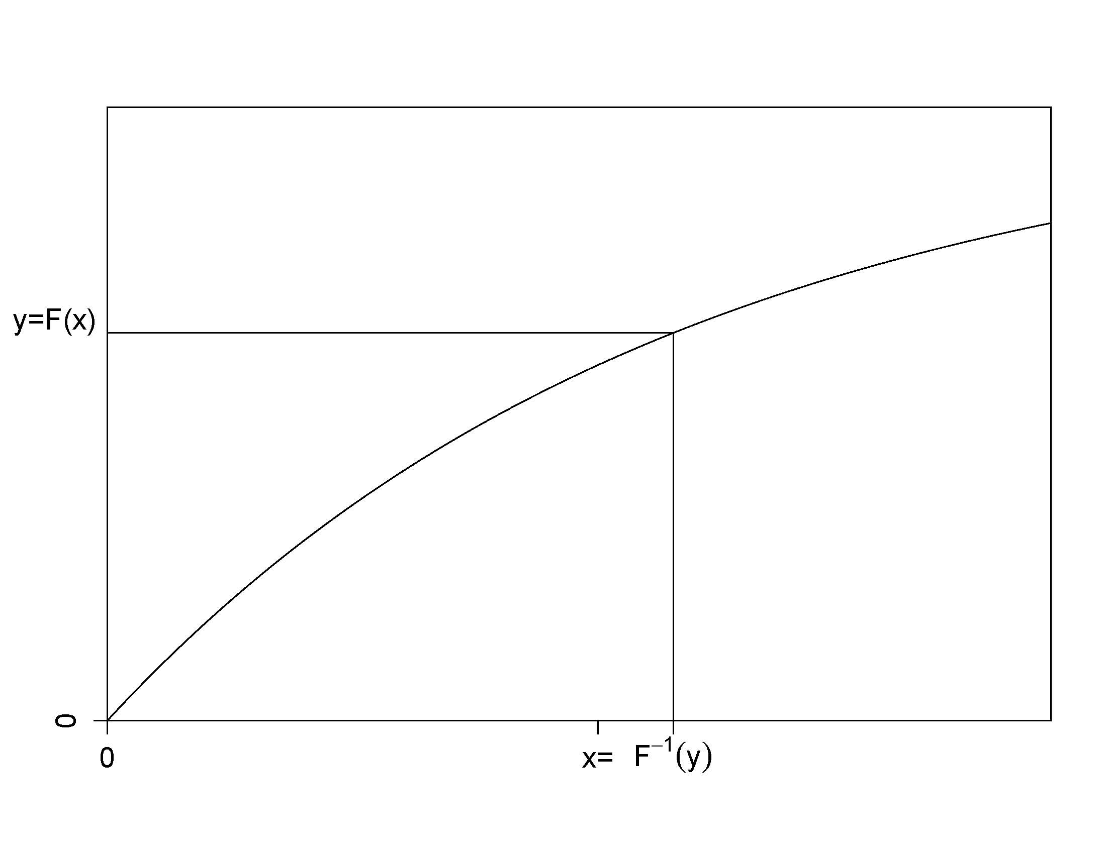
To interpret the result, recall that a distribution function, (F), is monotonically increasing and so the inverse function, (F^{-1}), is well-defined. The inverse distribution function (also known as the quantile function), is defined as
begin{eqnarray*}
F^{-1}(y) = inf_x { F(x) ge y } ,
end{eqnarray*}
where “(inf)” stands for “infinum”, or the greatest lower bound.
Here is a graph to help you visualize the inverse transform. When the random variable is continuous, the distribution function is strictly increasing and we can readily identify a unique inverse at each point of the distribution.
The inverse transform result is available when the underlying random variable is continuous, discrete or a mixture. Here is a series of examples to illustrate its scope of applications.
Exponential Distribution Example. Suppose that we would like to generate observations from an exponential distribution with scale parameter (theta) so that (F(x) = 1 – e^{-x/theta}). To compute the inverse transform, we can use the following steps:
begin{eqnarray*}
y = F(x) &Leftrightarrow& y = 1-e^{-x/theta}
&Leftrightarrow& -theta ln(1-y) = x = F^{-1}(y) .
end{eqnarray*}
Thus, if (U) has a uniform (0,1) distribution, then (X = -theta ln(1-U)) has an exponential distribution with parameter (theta).
Some Numbers. Take (theta = 10) and generate three random numbers to get
| (U) | 0.26321364 | 0.196884752 | 0.897884218 |
| (X = -10ln(1-U)) | 1.32658423 | 0.952221285 |