3 Simulating Regression Models

Being able to generate your own example data is an imporant tool. You know where your data came from, which puts you in a position to judge how well your analysis recovered the essential features of the data.

3.1 Simple Regression

You begin with an empty slate, then generate \(x\). This could be from any arbitrary data distribution, so here we will use a continuous uniform distribution. Next we generate the \(\beta\)s. Here we will just pick two arbitrary values, 10 and -0.5. Then we generate the \(\epsilon\) values. These come from a random Normal distribution with a mean of 0 and an arbitrary \(\sigma\), 1.5.

Finally, we combine all of these to generate \(y\). The model for which we are creating data is:

\[ y \sim N(10-0.5x, 1.5^2)\]

clear all
set obs 50 // an arbitrary _N

3.1.1 Generate Data

generate x = runiform(0,20)
generate b0 = 10
generate b1 = -0.5
generate e = rnormal(0, 1.5) // sigma == 1.5

generate y = b0 + b1*x + e

The first five observations look like this:

list * in 1/5, noobs

(Rather than generating so much repeated data, we will find more efficient ways of doing this in future examples.)

3.1.2 Plot the Data

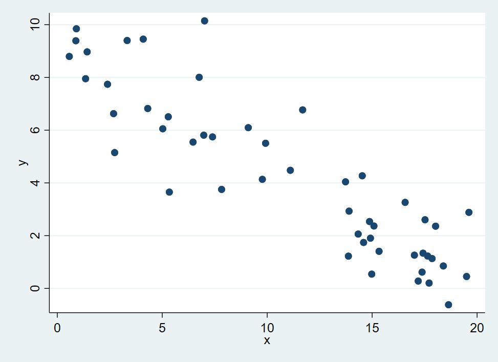
A scatter plot graphing \(y\) with \(x\):

graph twoway scatter y x

3.1.3 Plot the Random Component

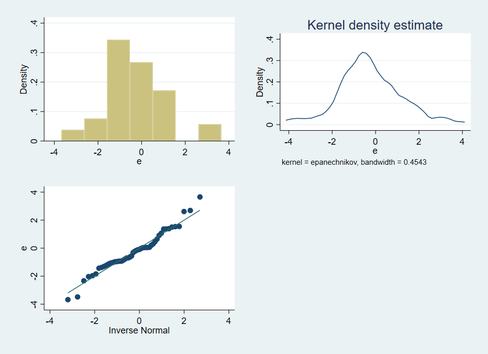
We might graph the random element, \(e\), in several different ways.

histogram e, name(h)
kdensity e, name(kd)
qnorm e, name(q)
graph combine h kd q

3.1.4 Plot the Model

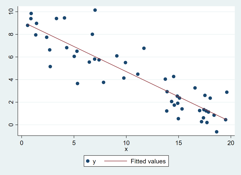
Then a graph including both the data and the regression line we are fitting is:

graph twoway (scatter y x) (lfit y x)

3.1.5 Regress

We can fit this model with the regress command in Stata:

regress y x
*anova y c.x // would fit the same model

      Source |       SS           df       MS      Number of obs   =        50
-------------+----------------------------------   F(1, 48)        =    187.78
       Model |  370.327761         1  370.327761   Prob > F        =    0.0000
    Residual |  94.6603772        48  1.97209119   R-squared       =    0.7964
-------------+----------------------------------   Adj R-squared   =    0.7922
       Total |  464.988138        49  9.48955383   Root MSE        =    1.4043

------------------------------------------------------------------------------
           y |      Coef.   Std. Err.      t    P>|t|     [95% Conf. Interval]
-------------+----------------------------------------------------------------
           x |  -.4440427   .0324037   -13.70   0.000    -.5091948   -.3788906
       _cons |   9.144904    .405187    22.57   0.000      8.33022    9.959587
------------------------------------------------------------------------------

3.1.6 Repeat

We can repeat this example numerous times by using the simulate command. This requires us to set up our data generation and model estimation as a program (essentially, a single Stata command).

program define example1, eclass
    clear
    set obs 25
    generate x = runiform(0,25)
    generate b0 = 10
    generate b1 = -0.5
    generate e = rnormal(0, 1.5) // sigma == 1.5
    generate y = b0 + b1*x + e

    regress y x
end

simulate b0=_b[_cons] b1=_b[x] e=e(rmse), reps(250) nodots: example1
summarize

      command:  example1
           b0:  _b[_cons]
           b1:  _b[x]
            e:  e(rmse)

    Variable |        Obs        Mean    Std. Dev.       Min        Max
-------------+---------------------------------------------------------
          b0 |        250    10.02846    .6277865   8.522183   11.82408
          b1 |        250   -.5025731    .0442147  -.6190096   -.356326
           e |        250    1.479487    .2249147   .9509845   2.075752

From here would could look at the distribution of b0 and b1.

3.2 Simple ANOVA (t-test)

A two group ANOVA is the same model as a two-group t-test.

For this example we’ll code \(group \in {0,1}\). The mean of \(y\) for each group is 0 and 2, respectively. And \(y\) has a \(\sigma=2\).

\[y \sim N(0+2*group, 2^2)\]

3.2.1 Generate Data

clear
set obs 50
generate group = _n > 25 // by observation number

generate y = rnormal(group*2, 2)

number of observations (_N) was 0, now 50

3.2.2 Plot the Data

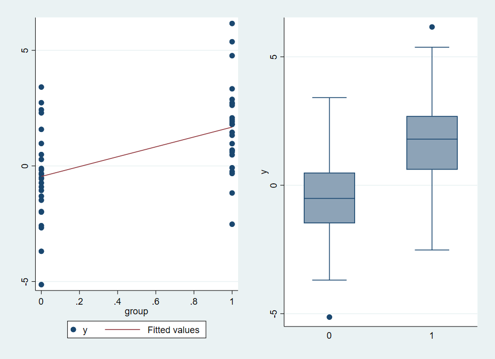
We can plot our data as a scatterplot. It is also common practice to graph this as a boxplot.

twoway (scatter y group) (lfit y group), name(s)
graph box y, over(group) name(b)
graph combine s b

(file ttplot.png written in PNG format)

3.2.3 regress

This is a model we could fit with several different commands.

ttest y, by(group)
oneway y group, mean
anova y group

As a regression, we would use

regress y i.group

      Source |       SS           df       MS      Number of obs   =        50
-------------+----------------------------------   F(1, 48)        =     14.36
       Model |  56.9630552         1  56.9630552   Prob > F        =    0.0004
    Residual |  190.443253        48  3.96756776   R-squared       =    0.2302
-------------+----------------------------------   Adj R-squared   =    0.2142
       Total |  247.406308        49  5.04910832   Root MSE        =    1.9919

------------------------------------------------------------------------------
           y |      Coef.   Std. Err.      t    P>|t|     [95% Conf. Interval]
-------------+----------------------------------------------------------------
     1.group |   2.134723   .5633875     3.79   0.000     1.001957     3.26749
       _cons |  -.4549388   .3983751    -1.14   0.259    -1.255926     .346048
------------------------------------------------------------------------------

Note the categorical (“factor”) variable prefix. In this particular example, because group has only the two levels, already coded 0 and 1, we could get away with skipping the prefix.

(The oneway and anova commands both assume group is a categorical variable. You could still add the prefix, for clarity.)