/* setup, proc reg requires numeric variables */
data class;
    set sashelp.class;
    female = sex eq "F";
run;Simple SAS Graphs with ODS
Over the many decades SAS has developed three distinct collections of graphics commands. The latest - and the most fully featured - is usually called ODS Graphics (Ouput Delivery System).
ODS graphics can be used in two ways. One is through PROC SGPLOT and several related ODS procedures. Another is through the graphics options built into most statistical procedures.
Using ODS graphics, many statistical procedures automatically create the graphs that are most commonly needed for a particular analysis. In addition, many more procedures have options to produce plots related to their analysis.
You can use ODS to:
- save statistical graphics in various graphics or document formats,
- select components of the statistical graphics output, and
- use styles and templates to customize the appearance of statistical graphics.
ODS for tables of statistical output is documented in Saving SAS Output Files.
Designing Your Own Plots and Charts
See Common SAS Plots for a quick start to using PROC SGPLOT. This will also illustrate how many of the statistical procedures can be used to produce the same (or nearly the same) graphs.
Automatic Graphics
The example below illustrates just how simple it is to generate graphics. The following statements invoke the REG procedure and fit a simple linear regression model.
/* automatic diagnostic graphs */
proc reg data=class;
    model height = age female;
    run; quit;
The REG Procedure
Model: MODEL1
Dependent Variable: Height
Number of Observations Read 19
Number of Observations Used 19
Analysis of Variance
Sum of Mean
Source DF Squares Square F Value Pr > F
Model 2 349.50473 174.75236 22.61 <.0001
Error 16 123.65948 7.72872
Corrected Total 18 473.16421
Root MSE 2.78006 R-Square 0.7387
Dependent Mean 62.33684 Adj R-Sq 0.7060
Coeff Var 4.45973
Parameter Estimates
Parameter Standard
Variable DF Estimate Error t Value Pr > |t|
Intercept 1 27.36034 5.95866 4.59 0.0003
Age 1 2.72759 0.43981 6.20 <.0001
female 1 -2.83621 1.27974 -2.22 0.0415With PROC REG, the graphical output automatically produced by ODS consists of a diagnostics panel, and a residual plots panel. These are shown below.
Model: MODEL1
Dependent Variable: Height
Optional Plots
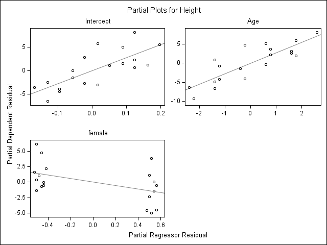
Many statistical procedures incorporate optional PLOT requests. For example, with PROC REG, you could request partial plots - a partial plot shows the effect of each variable after controlling for the other variables in the model (the slope is the same as the model coefficient).
To produce partial plots with PROC REG, add a partial option to the MODEL statement.
proc reg data=class;
    model height = age female / partial;
run; quit;Saving Graphics
By default, SAS includes these graphics as part of the HTML output it produces. However, all this output is deleted when you close your SAS session, including the graphics. To save graphics (and other output) you need to redirect output into a file using ODS commands.
If you save your output as a PDF, Word, or HTML5 file, the graphics are included within the file.
ods pdf file="example.pdf";
proc reg data=sashelp.class;
  model height = age;
  run;
ods pdf close;
If you save your output as an HTML file, the graphics are saved as separate graphics files that are linked to the HTML file.
ods html file="example.html";
proc reg data=sashelp.class;
  model height = age;
  run;
If you save your output as a text (listing) file, you must turn on ODS GRAPHICS, and then the graphics are saved as separate graphics files.
ods listing file="example.lst";
ods graphics on;
proc reg data=sashelp.class;
  model height = age;
  run;
Graphics File Formats
Each output document type has it’s own default graphics file type. You can specify a different file type, depending on the output destination. The most common defaults are PNG and SVG files.
To choose an alternative graphics file format, you use an ODS GRAPHICS statement. For example to save graphics as JPEG files, you might use
ods listing file="example.lst";
ods graphics on / outputfmt=jpeg;
proc reg data=sashelp.class;
  model height = age;
  run;
Customizing The Appearance of Your SAS Output
With ODS you can change the appearance of most of your SAS output. To change the overall look of your output, use ODS styles. To further customize the appearance and table of your output, you can change the templates SAS uses to generate output or even create your own templates. A brief overview of templates is provided in Redirecting and Customizing Tabular Output in SAS. For more detailed information, please refer to SAS's on-line manual.
ODS Styles
ODS styles control the overall look of your output. A style definition provides formatting information for specific visual aspects of your SAS output. For ODS graphics, this includes the appearance of line and marker properties in addition to font and color information.
You can specify a style using the style option in the ODS destination statement. Each style produces output with the same table, but with a somewhat different visual appearance. Of the SAS-supplied styles, SAS recommends four for use with ODS Graphics: ANALYSIS, DEFAULT, JOURNAL, and STATISTICAL. In the example below, the JOURNAL style is specified:
ods latex style=journal;

proc reg data=Class;
   model Weight = Height;
quit;

ods latex close;
Once you start using ODS you will find that you need details not contained in this overview document: see SAS's comprehensive ODS user guide.
Last Revised: 9/27/2024
