3 Working with the R Language
To write R scripts, it helps to be able to read the R documentation. We’ll begin with some of the jargon used to describe the R language and then look at the rules for writing R commands that the computer will be able to interpret.
Then we will examine some of the standard elements of the Help pages, and look at how new commands are added in the form of packages.
3.1 R Language Elements
The fundamental unit of work in R is the expression or statement. R evaluates statements.
Expressions are composed of data objects, functions, and special characters.
One of the most basic expressions is assigning data values to a name. Typical style would put one statement per line.
x <- rnorm(10, mean=5)
y <- rnorm(12, mean=7)
Let’s dig into the details.
xis the name of a data object<-is the assignment operator. Operators have a left-hand side and a right-hand side.rnorm()is a function, including the parentheses10andmean=5are function arguments, or parameters.meanis an argument name. The=is an assignment operator for function arguments.5is the value given for themeanargument.
You can think of each piece of an expression as a word, or token.
A token is generally a name (of a data object, a function, or an
argument), an operator (like <- or +), or another special
character like parentheses, brackets, and braces.
3.1.1 Capitalization
Capitalization matters. Try
X <- rnorm(3, mean=3)
x <- Rnorm(3, mean=3)
Error in Rnorm(3, mean = 3): could not find function "Rnorm"
x <- rnorm(3, Mean=3)
Error in rnorm(3, Mean = 3): unused argument (Mean = 3)
In the first statement, we get a new vector, X capitalized. Be careful!
While this is valid code, it might have been a typo!
In the second statement, we get an error about an unrecognized function - the function name should have been lower case.
In the third statement, we get an error about an unrecognized argument - the argument name should have been lower case.
If you decide to use capitalization when you name objects, try to do so in a consistent style.
3.1.2 White Space
White space between tokens does not matter, except for line breaks. White space used well makes your code much easier for humans to read and understand.
Try:
x<-rnorm(10,mean=5)
x <- rnorm ( 10 , mean = 5 )
These are both valid code. In there first statement, there is no white space at all. In the second statement, there is white space between every single token. Where you have one white space, you can have many white spaces.
Again, using white space will make your code easier for humans to read and understand, especially if you use it in a consistent way.
3.1.3 Line Breaks
An R statement may extend over more than one line. As long as an expression is incomplete at the end of a line, R will continue reading the next line before evaluating the statement.
Try this example:
x <-
  rnorm(5, mean=3)
This is valid code. In fact, if you highlight and run
just one line, the RStudio Console presents you with a +
prompt, indicating you have a dangling expression. (If
you use Ctrl-Enter, instead, RStudio reads both lines!)
A little caution is required with the placement of parentheses and operators: you may place an open parenthesis or an operator before a line break, but not after.
Compare these examples:
z <- 3 + 4
z <- 3
  + 4
[1] 4The first line is a complete statement, assigning the value 7 to z.
Written as above, the second line is also a complete statement, assigning the value 3 to z. Then the third line is simply a request to print the value 4.
3.1.5 Style
Try to write your code in a consistent and conventional manner. White space around operators make them easier to spot. White space between function arguments make them easier to distinguish. White space to indent blocks of code that run together makes it easier to see the flow of processing in a script.
Consistency makes your code easier to debug, and easier for people (your future self, colleagues, consultants) to read. You may find it helpful to consult an established style guide, such as The tidyverse style guide.
3.2 Using Help
RStudio makes it fairly easy to find documentation on most R functions. However, R documentation takes some practice to read.
The Help documentation is generally organized so that each function is documented on one page.
Of course, be sure to make use of the other materials published on the SSCC Website. If you are a member of the SSCC, you can also make an appointment with one of the statistical consultants to discuss your issue further.
3.2.1 RStudio’s Help Pane
The main way to navigate Help is to search. You can either search for the name of a specific function (if you already know it), or you can do a keyword search.
The RStudio Help pane is in the lower right of the workspace, tabbed with Files and Plots. It has two search boxes. The box on the upper right is used to find documentation pages, by function or keyword. The box toward the upper left is used to find keywords within the page you are currently looking at.
Let’s use the t.test function as an example.
If we didn’t already know the name of the function, we might search
by typing in “t-test” in the search box (and hitting the Enter key).
This brings up a list of documentation pages, including Help pages.
Scanning the list, we see stats::t.test Student's t-Test (stats
is the name of a package, but more on packages later). From
here we can click on the link and go to the documentation page.
Alternatively, if we know the function name, we can type “t.test” directly in the search box. As we type, we see a list of possible functions, and we can click on the one we want at any time.
3.2.2 Reading a Help Page
A single help page many document more than one function, and a function may work with several types of arguments (methods). This means that not everything documented on a given page is relevant to the task at hand: a big part of reading Help is figuring out which details matter, and which ones don’t.
The basic elements of a Help page are always the same:
- Description: a brief description
- Usage: a syntax diagram, showing argument names and default values
- Arguments: a more detailed description of the argument options
- Value: the kind of data returned by the function
Most Help pages also include:
- Details: some usage or arguments may require more detailed explanation
- See Also: possibly related functions
- Examples: working examples with comments, that you can try
3.2.3 Exercises - Using Help
Look up the Help for rnorm. There are four functions documented on this page.
- Which arguments does
rnormuse? - Create two random vectors,
v1andv2. Each should have a different number of data values, different means, and different standard deviations. Then perform a two-sample t-test. - Look up the Help for
mtcars, an example data set. What does the columnqsecmean? - Look up the Help for
meanand forcolMeans. Does the Help page make it clear what happens when you use themeanfunction with a data frame? ThecolMeansfunction?
3.3 Using Functions
As described in the last section, most functions take input in the form of arguments and return output in the form of a data object (the return “value”).
The arguments may be given in order (positionally), by name, or as a mix of both. Common style is to fill in the first argument positionally, and to give other arguments by name.
Consider the rnorm function. The help page tells us it’s
arguments are
rnorm(n, mean = 0, sd = 1)This function has three arguments, two of which also have default values.
If we use this function with one argument
rnorm(5)[1] -1.1851976 0.6877094 -1.3012967 0.7645003 -0.1166523the “5” in our
code is understood to be the first argument, n. Rather
than assigning n a value by it’s position in our code,
we could equally have specified it by name
rnorm(n=5)Now suppose we want our random numbers to come from a distribution with a mean of 10 and a standard deviation of 2. The clearest style would be to write
rnorm(5, mean=10, sd=2)[1] 11.688777 10.312569 12.095111 12.879219 8.525218It is also possible to give all the arguments by position or to name all the arguments.
rnorm(5, 10, 2)           # by position
rnorm(n=5, mean=10, sd=2) # by name
If we are using names, the arguments do not have to be in any order (although good style usually preserves the order anyway, for readability).
rnorm(sd=2, n=5, mean=10)As we have seen previously, the value assigned to a function argument can the the value give in another data object, or it can be the result of evaluating a sub-expression.
x <- 2
rnorm(5, mean=5*x, sd=x)
3.4 R Packages
R is available as a series of modules called packages, a few of which you downloaded and installed when you initially installed R.
Packages can contain all sorts of objects, but generally they are sources of new functions, data sets, example scripts, and documentation.
Anyone can develop and submit a package to CRAN, the central repository. CRAN packages must meet certain benchmarks to be accepted and distributed.
CRAN packages vary considerably in style and the quality of their documentation, even after meeting the CRAN benchmarks.
There are two main steps to using a package:
- installing the package on your computer
- telling R to use that package for objects (functions, data).
While you only need to install a package once, you need to tell R to use that package any time you start a new R session.
In the SSCC, you will find that there are many packages already installed for you. You can install or update packages yourself - these will automatically be installed in a folder on your U:\ drive.
3.4.1 What packages are already installed?
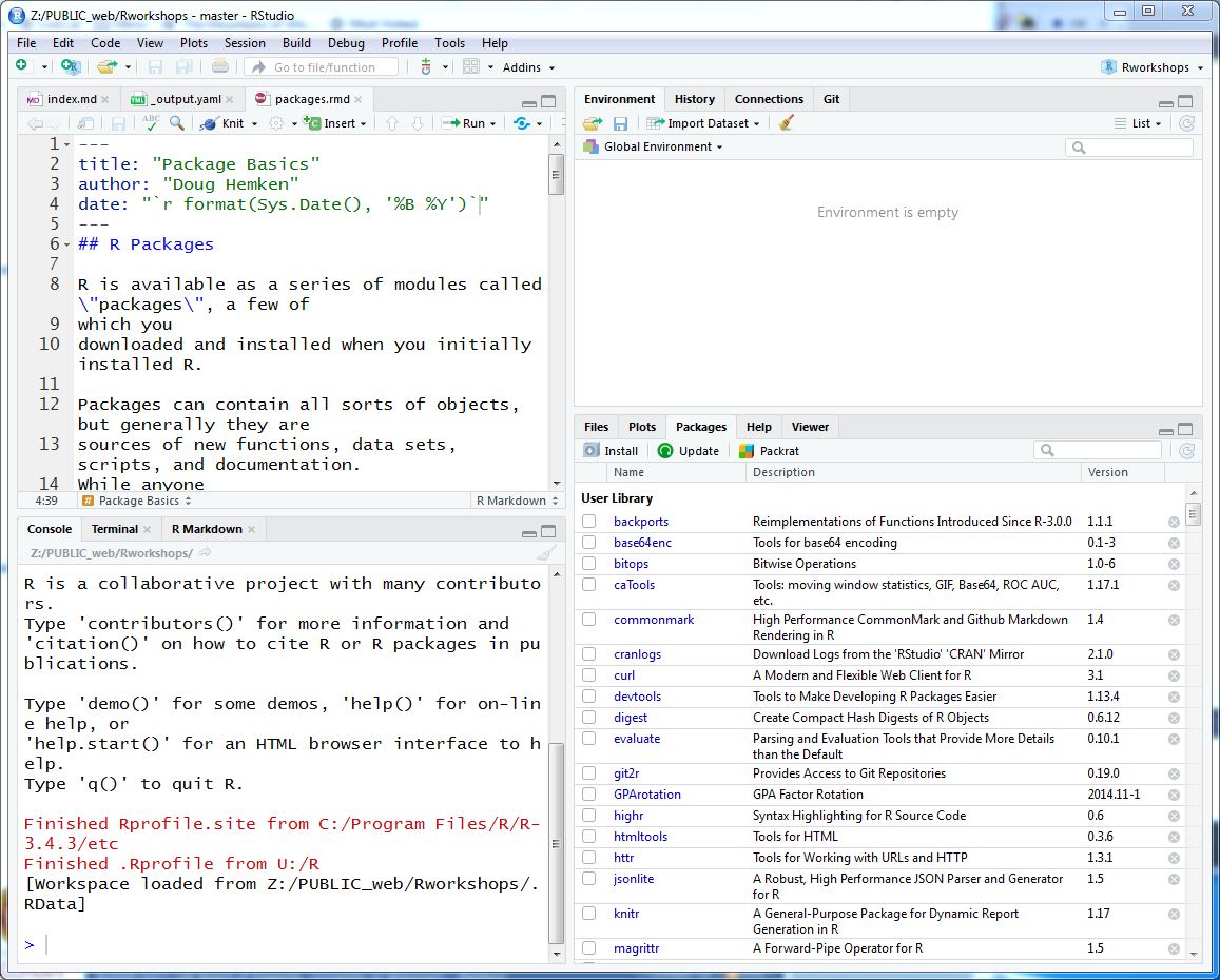
If you are working in RStudio you can see the installed packages in the Packages pane, tabbed in the lower right of RStudio with Files, Plots, and Help.
You can scroll through the list, or use the search box in the upper right of the pane. The search box works much like it does in Help.
You can click on a package name to see a Help page listing all of the functions and other objects in that package.
For example, suppose you were looking for documentation
on a function to read Stata data into R. If you thought it
might be in the foreign package you could
- search for the package
foreignin the Packages pane - click on the package name
- scroll to find the function you need in the list:
read.dta()(it doesn’t have “stata” in the function name, making it harder to search for) - click on
read.dta, and find yourself on the Help page
Try it!
3.4.2 Installing Additional Packages
You can install a package with the Install icon on the Packages toolbar. By default this installs packages from CRAN. If you have a package from another source in the form of a downloaded archive file, you can also install from that.
You can also install packages by using code. The following
code installs the faraway package from CRAN
(https://cloud.r-project.org/):
install.packages("faraway", repos="https://cloud.r-project.org/")Installing package into 'U:/R/4.0.5'
(as 'lib' is unspecified)package 'faraway' successfully unpacked and MD5 sums checked
The downloaded binary packages are in
C:\Users\hemken\AppData\Local\Temp\Rtmp0QGxob\downloaded_packages3.4.3 Using a Package
To actually use the material in the package you must load it
using the library function:
library(faraway)

summary(hsb)       # the data "hsb" is in the package
id gender race ses schtyp prog
Min. : 1.00 female:109 african-amer: 20 high :58 private: 32 academic:105
1st Qu.: 50.75 male : 91 asian : 11 low :47 public :168 general : 45
Median :100.50 hispanic : 24 middle:95 vocation: 50
Mean :100.50 white :145
3rd Qu.:150.25
Max. :200.00
read write math science socst
Min. :28.00 Min. :31.00 Min. :33.00 Min. :26.00 Min. :26.00
1st Qu.:44.00 1st Qu.:45.75 1st Qu.:45.00 1st Qu.:44.00 1st Qu.:46.00
Median :50.00 Median :54.00 Median :52.00 Median :53.00 Median :52.00
Mean :52.23 Mean :52.77 Mean :52.65 Mean :51.85 Mean :52.41
3rd Qu.:60.00 3rd Qu.:60.00 3rd Qu.:59.00 3rd Qu.:58.00 3rd Qu.:61.00
Max. :76.00 Max. :67.00 Max. :75.00 Max. :74.00 Max. :71.00 3.4.4 Undoing things
detach(package:faraway, unload=TRUE) # disassociates the package from your current session
remove.packages("faraway") # removes a package from your computer
Removing package from 'U:/R/4.0.5'
(as 'lib' is unspecified)3.4.5 Exercises - Installing Packages
- Install and load the package
magrittr. This package is the source of a pipe operator,%>%, which can be used to write many R statements in left-to-right form rather than in nested form.
Using this package, rewrite t.test(rnorm(15, mean=5)) as
rnorm(15, mean=5) %>% t.testand verify that both produce the same output.
- Install the package
dplyr. This package contains many functions that are useful for manipulating data.
Using this package, put the rows of the mtcars data in ascending
order by mpg.
mtcars %>% arrange(mpg)
3.1.4 Comments
We use comments in our code to write notes for humans to read, and to disable sections of code (perhaps temporarily).
The
#symbol is the comment token. Any text on a line after a#character is ignored by R.Try this example, which contains two comments: