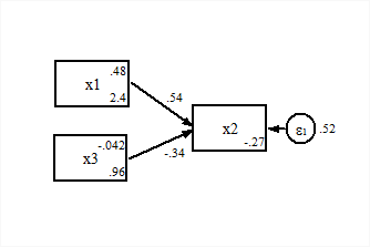
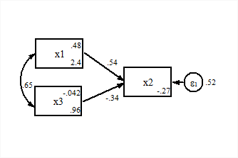
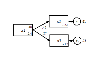
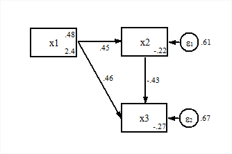
Using the SEM Builder
Stata has a graphical user interface for specifying and estimating structural equation models, call the "Builder". From the menus, click on Statistics -> SEM -> Model building and estimation.
SEM menu
Using the SEM model objects on the left, build a model. For example, click on the rectangular box near the top of the object list, then click once on the blank model canvas in two separate places, in order to include two observed variables in your model. Next, click on the rightward-pointing arrow, the path object, and click once on each observed variable box to connect them. Finally, click on the selection icon at the top of the model object list and click on one of the observed variable boxes. In the bar above the model canvas you can fill in the variable name. Do this for the other observed variable as well. The set up should look like this:
SEM model
Now you can click on the Estimate button in the top toolbar (the Execute icon). The sem command for your model runs in the main Stata workspace, and some of the parameter estimates are displayed on the Builder model.
SEM estimates
Builder models and sem commands
Notice that running models from the Builder generates Stata sem commands which you can save in a *.do file, and also produces all the same output that using the command does, which you can save in a *.log file.
There is no way to go in the other direction, however. That is, there is no way to have an sem command automatically produce a Builder diagram.
Saving Models and Diagrams
You can save your model specification and estimates in their graphical for as a Stata stem file. This allows you to reopen your model and do further work with it in a later Stata session.
You can also save your model diagram in whatever state it is in (pre- or post-estimation).
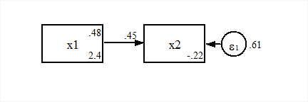
Saved diagram
