Models can be expressed in many alternative coordinate systems. We usually pick a coordinate system, a base of reference, that will be convenient both mathematically and for the sake of interpretation, given the analytical task at hand.
On occasion, it is useful to be able to change our base of reference, to look at the same model from another point of view. Often, this is done by recoding the data upon which our model is based. With the data expressed in a new coordinate system, a freshly estimated model is then interpreted on the new basis.
Where the model takes a particularly long time to run, or where we may no longer have access to the original data, a more efficient or perhaps the only means of proceeding is through post-estimation translations, a.k.a. reparameterization. This also shows us a thing or two about the relationship between different model parameterizations.
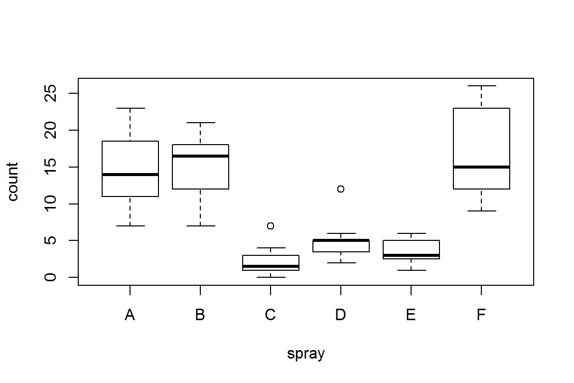
As an example, look at the data set InsectSprays. The data give counts of dead insects in experimental plots, using six different sprays.
plot(count~spray, InsectSprays)
Consider the following two ANOVA models, one expressed in reference form, the other expressed in effects form. The reference form is parameterized as an intercept that is the mean count for the first category of sprays, and the remaining parameters are differences in the means of each remaining category from the first. In other words, we have \[y=\beta_0+\beta_i x_i\] with \(\beta_0\) as the mean count of the first spray, and the \(\beta_i\) as the differences in the mean between each remaining spray and the first spray. \(y\) is the predicted value, the mean, for each spray, and the \(x_i\) are indictors for each spray.
The effects form is parameterized as a grand mean (balanced) of all categories, and the remaining parameters are the differences in the means of first five categories from the grand mean. We can use the same formula as above, \[y=\beta_0+\beta_i x_i\] but here we give the symbols different meanings. Now \(\beta_0\) is the grand mean of all the sprays, the mean of the spray means. The \(\beta_i\) are now the differences between the grand mean and the mean of each spray (except one, which is dropped as redundant). \(y\) is still the predicted value for each spray. The \(x_i\) are coded 1 for belonging to the indicated spray, -1 for belonging to the dropped spray, or 0.
# model 1
contrasts(InsectSprays$spray)
## B C D E F
## A 0 0 0 0 0
## B 1 0 0 0 0
## C 0 1 0 0 0
## D 0 0 1 0 0
## E 0 0 0 1 0
## F 0 0 0 0 1(B1 <- coef(lm(count~spray, InsectSprays)))## (Intercept) sprayB sprayC sprayD sprayE sprayF
## 14.5000000 0.8333333 -12.4166667 -9.5833333 -11.0000000 2.1666667# model 2
contrasts(InsectSprays$spray) <- contr.sum
contrasts(InsectSprays$spray)## [,1] [,2] [,3] [,4] [,5]
## A 1 0 0 0 0
## B 0 1 0 0 0
## C 0 0 1 0 0
## D 0 0 0 1 0
## E 0 0 0 0 1
## F -1 -1 -1 -1 -1coef(lm(count~spray, InsectSprays))## (Intercept) spray1 spray2 spray3 spray4 spray5
## 9.500000 5.000000 5.833333 -7.416667 -4.583333 -6.000000These are, in a strong sense, the same model: they produce the same fitted and residual values, and have the same overall fit statistics.
In fact the coefficients and precision matrix for each model can be derived as a linear transformation of the other. To make this easiser to follow, we first ensure that these models are expressed in terms of the same levels (sprays).
To have both models in terms of the same levels, we will have to rearrange the levels of one model: the first model was expressed in terms of levels B through F, while the second was expressed in terms of A through E. This is an important technical detail, easy to miss if you are just skimming the results!
Releveling model 2:
# model 2 revised
InsectSprays$spray <- factor(InsectSprays$spray,
                    levels=c("B", "C", "D", "E", "F","A"))
contrasts(InsectSprays$spray) <- contr.sum
(B2 <- coef(lm(count~spray, InsectSprays)))
## (Intercept) spray1 spray2 spray3 spray4 spray5
## 9.500000 5.833333 -7.416667 -4.583333 -6.000000 7.166667Consider the linear transformation defined by the matrix A:
# transform reference coding to effects coding
A # the linear transformation
## [,1] [,2] [,3] [,4] [,5] [,6]
## [1,] 1 0.1666667 0.1666667 0.1666667 0.1666667 0.1666667
## [2,] 0 0.8333333 -0.1666667 -0.1666667 -0.1666667 -0.1666667
## [3,] 0 -0.1666667 0.8333333 -0.1666667 -0.1666667 -0.1666667
## [4,] 0 -0.1666667 -0.1666667 0.8333333 -0.1666667 -0.1666667
## [5,] 0 -0.1666667 -0.1666667 -0.1666667 0.8333333 -0.1666667
## [6,] 0 -0.1666667 -0.1666667 -0.1666667 -0.1666667 0.8333333t(A %*%B1) # the transformed coefficients## [,1] [,2] [,3] [,4] [,5] [,6]
## [1,] 9.5 5.833333 -7.416667 -4.583333 -6 7.166667B2## (Intercept) spray1 spray2 spray3 spray4 spray5
## 9.500000 5.833333 -7.416667 -4.583333 -6.000000 7.166667And the inverse transformation
(Ainv <- solve(A))## [,1] [,2] [,3] [,4] [,5] [,6]
## [1,] 1 -1 -1 -1 -1 -1
## [2,] 0 2 1 1 1 1
## [3,] 0 1 2 1 1 1
## [4,] 0 1 1 2 1 1
## [5,] 0 1 1 1 2 1
## [6,] 0 1 1 1 1 2t(Ainv %*% B2)## [,1] [,2] [,3] [,4] [,5] [,6]
## [1,] 14.5 0.8333333 -12.41667 -9.583333 -11 2.166667B1## (Intercept) sprayB sprayC sprayD sprayE sprayF
## 14.5000000 0.8333333 -12.4166667 -9.5833333 -11.0000000 2.1666667Inspection of the vcov transformation is left as a coding exercise.
This particular pair of transformations takes a very regular form, which depends only on the number of levels.
A reference-to-effects transformation of an arbitrary number of levels can be found with the following function
ref2eff <- function(n) {
  stopifnot(n>=2 & length(n)==1 & is.integer(n))
  trans <- matrix(-1/n, nrow=n, ncol=n)
  trans[1,1] <- 1
  diag(trans[2:n,2:n]) <- (n-1)/n
  trans[1,2:n] <- 1/n
  trans[2:n,1] <- 0
  return(trans)
}

ref2eff(5L)
## [,1] [,2] [,3] [,4] [,5]
## [1,] 1 0.2 0.2 0.2 0.2
## [2,] 0 0.8 -0.2 -0.2 -0.2
## [3,] 0 -0.2 0.8 -0.2 -0.2
## [4,] 0 -0.2 -0.2 0.8 -0.2
## [5,] 0 -0.2 -0.2 -0.2 0.8Likewise, an effects to reference transformation can be found with
eff2ref <- function(n) {
  stopifnot(n>=2 & length(n)==1 & is.integer(n))
  trans <- matrix(1, nrow=n, ncol=n)
  diag(trans[2:n,2:n]) <- 2
  trans[1,2:n] <- -1
  trans[2:n,1] <- 0
  return(trans)
}

eff2ref(5L)
## [,1] [,2] [,3] [,4] [,5]
## [1,] 1 -1 -1 -1 -1
## [2,] 0 2 1 1 1
## [3,] 0 1 2 1 1
## [4,] 0 1 1 2 1
## [5,] 0 1 1 1 2Other variables can be added to these models, and the transformation takes a modified block form where the additional variables are additive, and takes a Kronecker product form where the additional variables include interaction terms. (The additive form can be seen as a sparse representation of the full factorial version.)