Overlay scatter and scatteri
Then we overlay the scatterplot and the immediate scatterplot of the single point.
twoway (scatter mpg price) (scatteri `Y' `X', msymbol(D))The msymbol(D) gives us a large, diamond-shaped point marker.
There are a couple of approaches one could take to add a single point to a scatterplot. One is to overlay the scatterplot with the plot produced by scatteri, an immediate scatterplot.
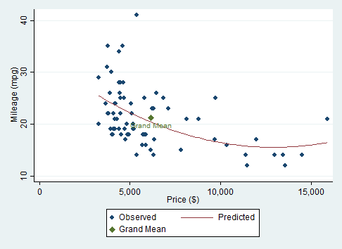
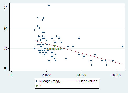
In this example, we will plot the overall mean in both the \(x\) and the \(y\) variables. A linear regression of \(y\) on \(x\) always passes through this point. A regression with higher-order terms seldom passes through this point!
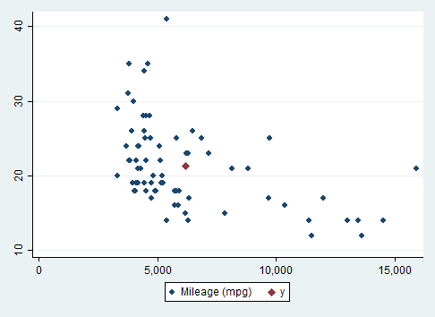
First we identify the mean values of \(y\) and \(x\) and save them as local macro variables.
  sysuse auto
  summarize price, meanonly
  local X = r(mean)
  summarize mpg, meanonly
local Y = r(mean)Then we overlay the scatterplot and the immediate scatterplot of the single point.
twoway (scatter mpg price) (scatteri `Y' `X', msymbol(D))The msymbol(D) gives us a large, diamond-shaped point marker.
  twoway (scatter mpg price)(lfit mpg price) ///
    (scatteri `Y' `X' (6) "Grand Mean", msymbol(D))
The "(6)" is a clock position for the point label.
  twoway (scatter mpg price)(qfit mpg price) ///
    (scatteri `Y' `X' (6) "Grand Mean", msymbol(D)), ///
    xtitle("Price ($)") ytitle("Mileage (mpg)") ///
    legend(order(1 "Observed" 2 "Predicted" 3 "Grand Mean"))
Here we can see that the regression line misses the grand mean.