Proc Step
With the data in SAS format, we can use various statistical PROCs to analyze the data.
Our first three questions can be answered with a single PROC MEANS.
proc means data=MendotaIce; * simple descriptive analysis;
    var days icein iceout;
    run;
The MEANS Procedure
Variable N Mean Std Dev Minimum Maximum
--------------------------------------------------------------------------
Days 163 102.5092025 19.4987711 21.0000000 161.0000000
icein 172 -9.9883721 12.8700152 -39.0000000 63.0000000
iceout 170 88.1823529 23.3533884 -24.0000000 125.0000000
--------------------------------------------------------------------------Over the last 150+ years, the average duration of ice cover has been 103 days, which gives us a substantial ice fishing season. The lake typically ices over 10 days before 1 January, or just as finals are ending. The ice usually breaks up around the 89th day of the year.
We could apply our date formats to interpret these results more easily.
                              icein    iceout

                              22DEC    29MAR
To see the distributions of the duration of ice cover, we can use a PROC step that produces graphs.
proc sgplot data=MendotaIce; * histograms;
    histogram days;
    run;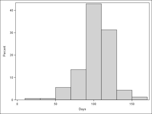
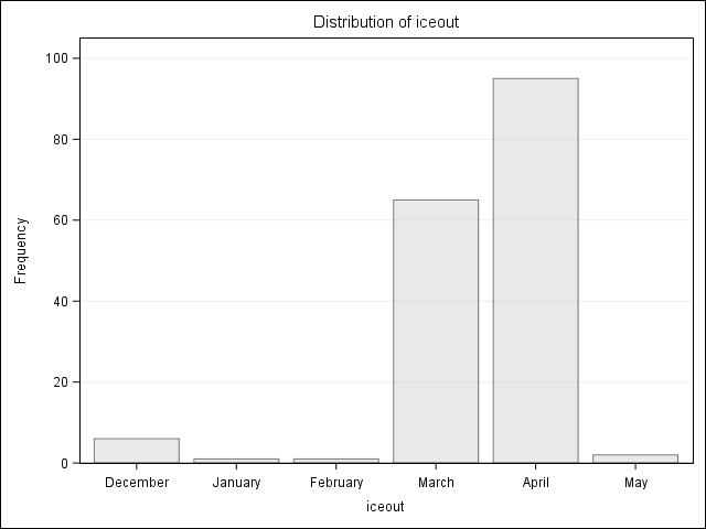
Many procedures produce both tables and plots. To look at the distribution of ice out by month we could do this:
proc freq data=MendotaIce; * frequency, by month;
    tables iceout / plots=freqplot;
    format iceout monname.;
run;| iceout | Frequency | Percent |
Cumulative Frequency |
Cumulative Percent |
|---|---|---|---|---|
| December | 6 | 3.53 | 6 | 3.53 |
| January | 1 | 0.59 | 7 | 4.12 |
| February | 1 | 0.59 | 8 | 4.71 |
| March | 65 | 38.24 | 73 | 42.94 |
| April | 95 | 55.88 | 168 | 98.82 |
| May | 2 | 1.18 | 170 | 100.00 |
| Frequency Missing = 4 | ||||
title "Days of Ice Cover";
title2 "Lake Mendota";

proc reg data=MendotaIce; * modeling yearly change in ice cover;
    model days = year;
    run; quit;
Days of Ice Cover
Lake Mendota
The REG Procedure
Model: MODEL1
Dependent Variable: Days
Number of Observations Read 174
Number of Observations Used 163
Number of Observations with Missing Values 11
Analysis of Variance
Sum of Mean
Source DF Squares Square F Value Pr > F
Model 1 13111 13111 43.54 <.0001
Error 161 48482 301.13134
Corrected Total 162 61593
Root MSE 17.35314 R-Square 0.2129
Dependent Mean 102.50920 Adj R-Sq 0.2080
Coeff Var 16.92837
Parameter Estimates
Parameter Standard
Variable DF Estimate Error t Value Pr > |t|
Intercept 1 471.70618 55.96971 8.43 <.0001
year 1 -0.19060 0.02889 -6.60 <.0001title;
data recentered;
set mendotaice;
yearc = year-2019;
run;
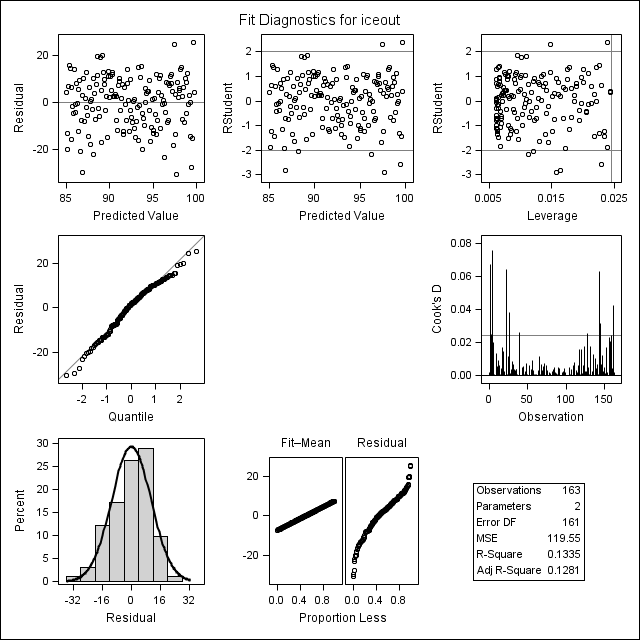
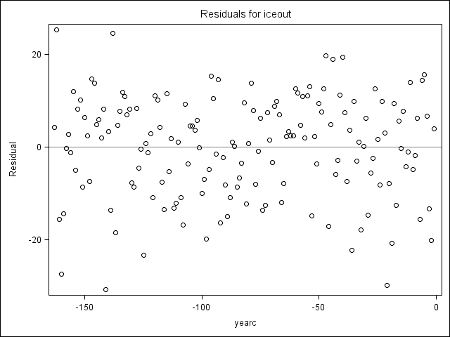
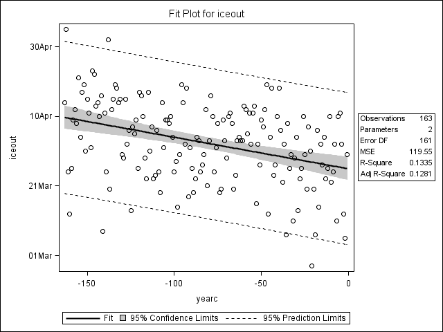
proc reg data=recentered; * modeling yearly change in ice cover;
model iceout = yearc;
where days ne .;
run; quit;
Model: MODEL1
Dependent Variable: iceout
| Number of Observations Read | 163 |
|---|---|
| Number of Observations Used | 163 |
| Analysis of Variance | |||||
|---|---|---|---|---|---|
| Source | DF |
Sum of Squares |
Mean Square |
F Value | Pr > F |
| Model | 1 | 2966.07226 | 2966.07226 | 24.81 | <.0001 |
| Error | 161 | 19248 | 119.55014 | ||
| Corrected Total | 162 | 22214 | |||
| Root MSE | 10.93390 | R-Square | 0.1335 |
|---|---|---|---|
| Dependent Mean | 92.36196 | Adj R-Sq | 0.1281 |
| Coeff Var | 11.83810 |
| Parameter Estimates | |||||
|---|---|---|---|---|---|
| Variable | DF |
Parameter Estimate |
Standard Error |
t Value | Pr > |t| |
| Intercept | 1 | 84.92797 | 1.72073 | 49.36 | <.0001 |
| yearc | 1 | -0.09066 | 0.01820 | -4.98 | <.0001 |
Model: MODEL1
Dependent Variable: iceout
2          data _null_;
3           mu=86;
4           ucl = mu + 1.96*10.86;
5           lcl = mu - 1.96*10.86;
6           put mu date.;
7           put lcl date.;
8           put ucl date.;
9           run;

27MAR60
05MAR60
17APR60
NOTE: DATA statement used (Total process time):
      real time           0.00 seconds
      cpu time            0.00 seconds
                                                                          1
                                           09:44 Tuesday, February 26, 2019

                             The REG Procedure
                               Model: MODEL1
                        Dependent Variable: iceout

                  Number of Observations Read         163
                  Number of Observations Used         163

                           Analysis of Variance

                                   Sum of          Mean
 Source                  DF       Squares        Square   F Value   Pr > F

 Model                    1    2966.07226    2966.07226     24.81   <.0001
 Error                  161         19248     119.55014
 Corrected Total        162         22214

           Root MSE             10.93390    R-Square     0.1335
           Dependent Mean       92.36196    Adj R-Sq     0.1281
           Coeff Var            11.83810

                           Parameter Estimates

                        Parameter       Standard
   Variable     DF       Estimate          Error    t Value    Pr > |t|

   Intercept     1       84.92797        1.72073      49.36      <.0001
   yearc         1       -0.09066        0.01820      -4.98      <.0001
proc reg data=recentered; * modeling yearly change in ice cover;
model open = yearc;
where days ne .;
run; quit; 1
09:44 Tuesday, February 26, 2019
The REG Procedure
Model: MODEL1
Dependent Variable: iceout
Number of Observations Read 163
Number of Observations Used 163
Analysis of Variance
Sum of Mean
Source DF Squares Square F Value Pr > F
Model 1 2966.07226 2966.07226 24.81 <.0001
Error 161 19248 119.55014
Corrected Total 162 22214
Root MSE 10.93390 R-Square 0.1335
Dependent Mean 92.36196 Adj R-Sq 0.1281
Coeff Var 11.83810
Parameter Estimates
Parameter Standard
Variable DF Estimate Error t Value Pr > |t|
Intercept 1 84.92797 1.72073 49.36 <.0001
yearc 1 -0.09066 0.01820 -4.98 <.0001
The REG Procedure
Model: MODEL1
Dependent Variable: open
Number of Observations Read 163
Number of Observations Used 163
Analysis of Variance
Sum of Mean
Source DF Squares Square F Value Pr > F
Model 1 48118519693 48118519693 4.009E8 <.0001
Error 161 19325 120.02840
Corrected Total 162 48118539017
Root MSE 10.95575 R-Square 1.0000
Dependent Mean -8307.74233 Adj R-Sq 1.0000
Coeff Var -0.13187
Parameter Estimates
Parameter Standard
Variable DF Estimate Error t Value Pr > |t|
Intercept 1 21635 1.72417 12547.9 <.0001
yearc 1 365.15186 0.01824 20022.3 <.00012 data _null_;
3 mu=20540;
4 ucl = mu + 1.96*10.88;
5 lcl = mu - 1.96*10.88;
6 put mu date9.;
7 put lcl date.;
8 put ucl date.;
9 run;
27MAR2016
05MAR16
17APR16
NOTE: DATA statement used (Total process time):
real time 0.00 seconds
cpu time 0.00 seconds
                                                                          1
                                           09:44 Tuesday, February 26, 2019

                             The REG Procedure
                               Model: MODEL1
                        Dependent Variable: iceout

                  Number of Observations Read         163
                  Number of Observations Used         163

                           Analysis of Variance

                                   Sum of          Mean
 Source                  DF       Squares        Square   F Value   Pr > F

 Model                    1    2966.07226    2966.07226     24.81   <.0001
 Error                  161         19248     119.55014
 Corrected Total        162         22214

           Root MSE             10.93390    R-Square     0.1335
           Dependent Mean       92.36196    Adj R-Sq     0.1281
           Coeff Var            11.83810

                           Parameter Estimates

                        Parameter       Standard
   Variable     DF       Estimate          Error    t Value    Pr > |t|

   Intercept     1       84.92797        1.72073      49.36      <.0001
   yearc         1       -0.09066        0.01820      -4.98      <.0001