Text Results
Examining text results is pretty obvious: output from R commands is “printed” to the Console by default.
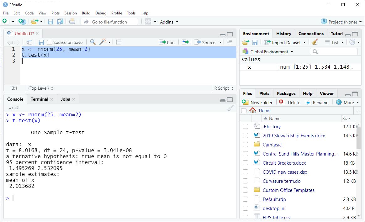
We can use the output from our last exercise as an example.
    x <- rnorm(25, mean=2)
    t.test(x)
You can resize your Console pane to see more (or less) of your output at once. The width of your Console affects where the lines of print output break, so adjust this before you run your commands.
The Console is a “buffer” that only holds 1000 lines of output. With a huge amount of output you cannot scroll back to the beginning. We deal with this by automatically saving output.
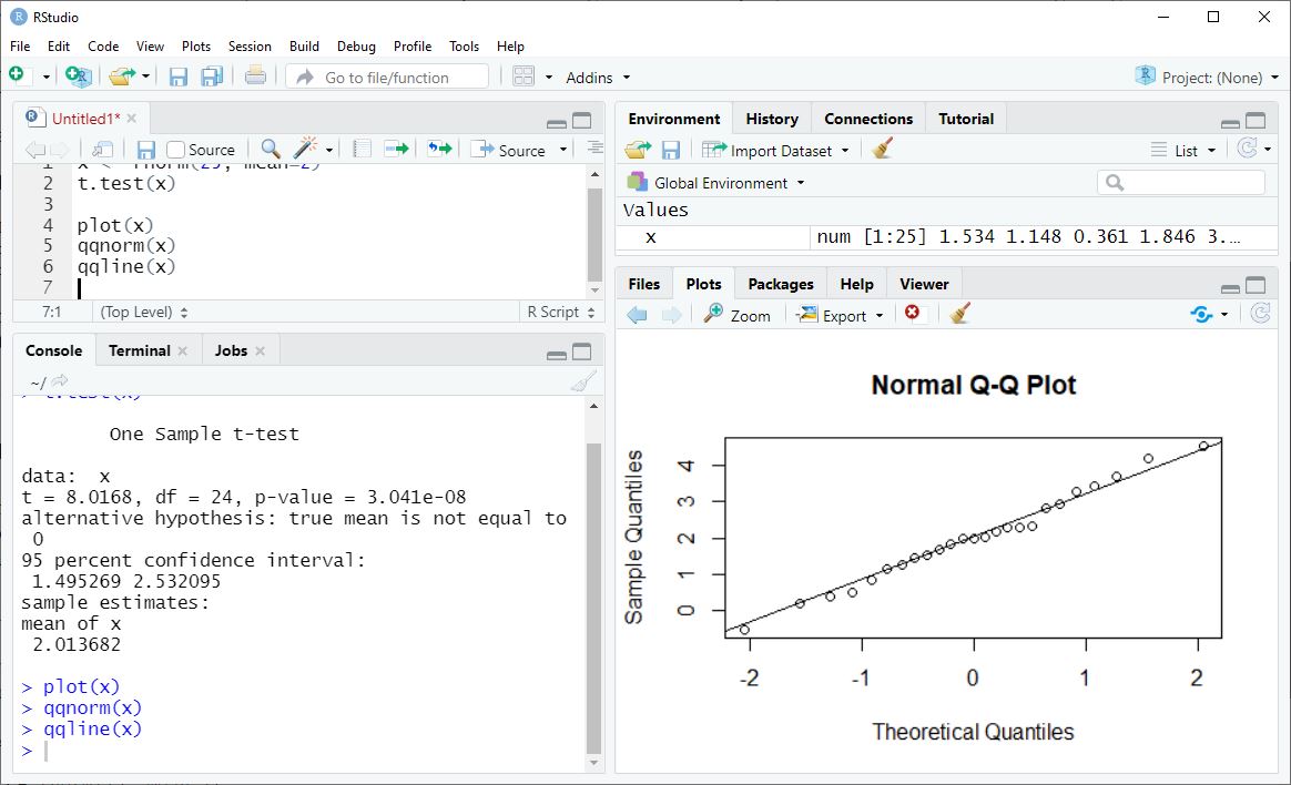
Graphs
Graphs appear in the Plots pane, in the lower right of the RStudio workspace.
Plot the data from our last exercise as an example. We’ll do two plots.
    plot(x)
    qqnorm(x)
    qqline(x)
Like the Console, the Plots pane can be resized. This changes the look of the plot (the size and the aspect ratio). You can also pop a graph into a separate window with the Zoom button in the Plots toolbar.
If you have created more than one graph, you can use the left and right arrows in the Plots toolbar to scroll among your graphs.
Examining Data
Looking at data values is a little more complicated, because data comes in many forms in R. We will discuss the varieties of R data in more depth later, but for now there are three main strategies for examining data values and properties: the Environment pane, printing to the Console, and viewing data frames and lists.
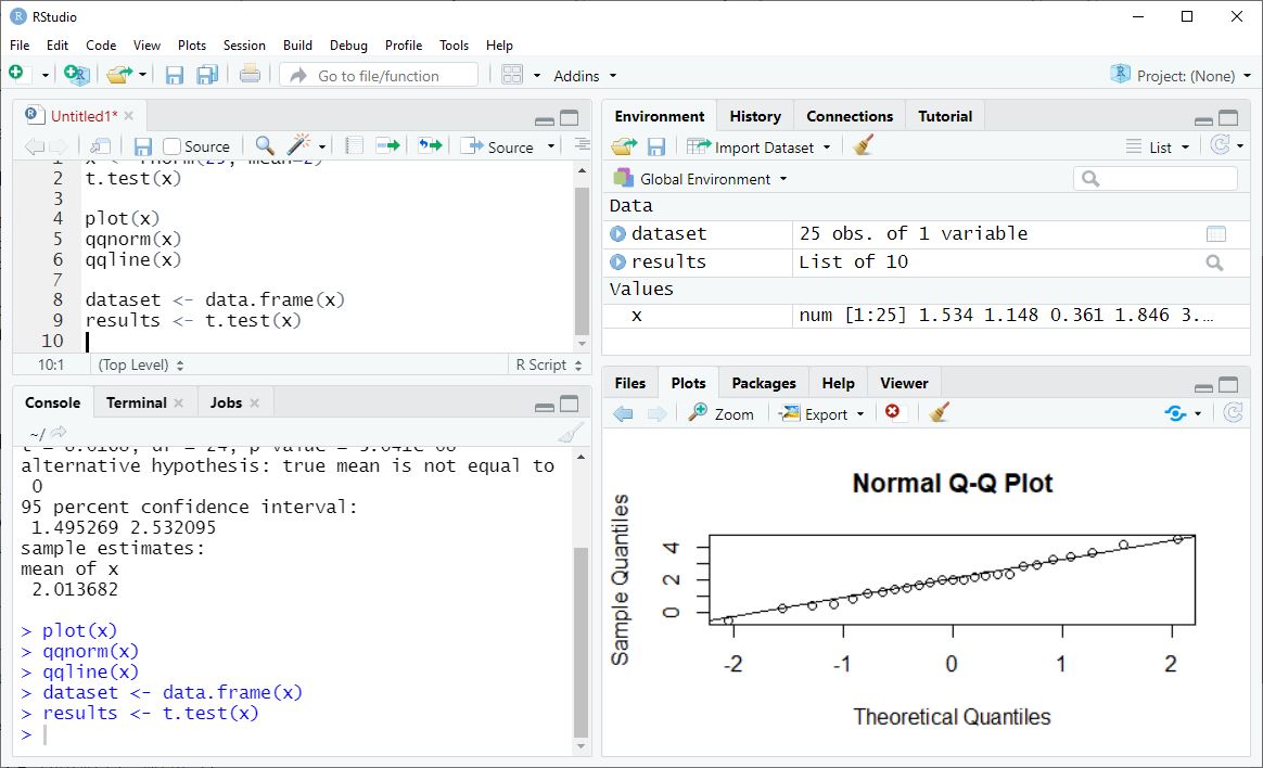
Environment Pane
The Environment pane in the upper right of the RStudio workspace shows the names of any data objects currently available in your computer’s memory.
As examples, let’s save our x data as a data frame, and also save our t.test() results as data.
    x <- rnorm(25, mean=2)
    dataset <- data.frame(x)
    results <- t.test(x)
Here, we see that x is a numeric vector with 25 observations, and we can see a few of the data values. For more complicated objects like dataset and results, we can click on the blue arrow next to the name to see more details of what is inside each object, including some data values.
Viewing Data Frames and Lists
If you double-click on the name of a data frame or list object in the Environment pane, a window opens in the Script area of RStudio. For a data frame this gives you a spreadsheet-like view of the data values. For a list, it gives you a somewhat cleaner way to browse the data elements there.
Printing Data
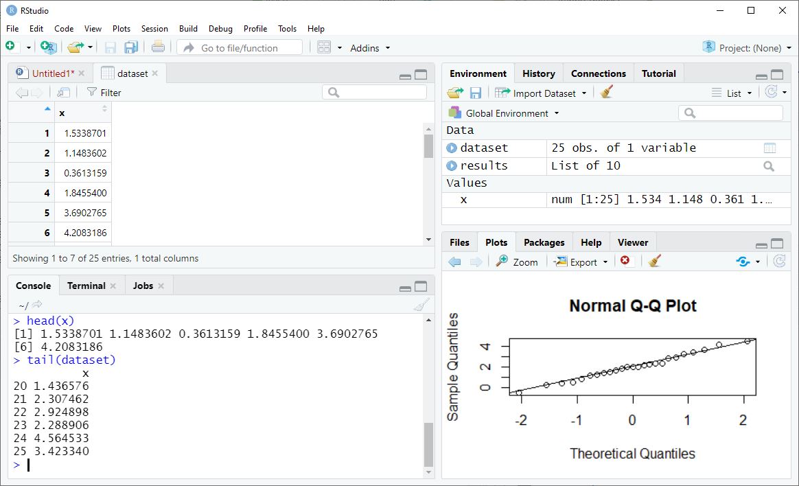
For basic data objects, printing them will show you the data values. To see just a few of the data values, use the head() or tail() functions.
head(x)
[1] 2.430514 3.364006 1.146390 2.776423 1.164514 2.235336
tail(dataset)
          x
20 1.723786
21 0.442435
22 1.996683
23 3.556930
24 1.455734
25 3.071782
How an object is printed depends on its class. So printing a data object like results does not actually simply list the data elements it stores. To see the actual data values being stored typically requires extracting or coercing the data object to print the elementary data values - topics for later.
class(results) <- NULL
results
$statistic
      t
10.4086

$parameter
df
24

$p.value
[1] 2.235727e-10

$conf.int
[1] 1.742839 2.604954
attr(,"conf.level")
[1] 0.95

$estimate
mean of x
 2.173897

$null.value
mean
   0

$stderr
[1] 0.2088559

$alternative
[1] "two.sided"

$method
[1] "One Sample t-test"

$data.name
[1] "x"